Open access

Testing unmanned aircraft systems for salmon spawning surveys

Publication: FACETS
9 November 2016

Abstract

Unmanned aircraft systems (UASs) were tested for counting Chinook salmon (Oncorhynchus tshawytscha) redds as a more accurate, safer alternative to manned helicopter flights. Counting redds from the helicopter was less expensive and time consuming, but of the total redds counted at selected sites with a UAS, an average (± SD) of only 77% ± 14% was counted from the helicopter. A river-wide census of redds was not possible with a UAS because the study area was too large for the single field crew to survey. Simulation analyses were used to compare stratified random sampling (STRS) and sampling proportional to size (PPS) for estimating annual total redd counts from data collected with a UAS. The STRS estimates were more accurate and precise, whereas the PPS estimates, though biased, had 95% CIs that included the observed redd count more frequently. We strongly recommend that researchers conduct simulation analyses to evaluate alternative survey sampling methods if they are considering replacing census counts made from manned aircraft with counts estimated from data collected with a UAS. We conclude that UAS application reduces the risk inherent to manned aircraft flights, but the reduction in risk can come at the cost of estimates of population parameters that can sometimes be inaccurate and lack 95% CI coverage.

Introduction

Salmon redds (i.e., nests) can be easy to see because they are relatively large and generally appear as regular- or irregular-shaped oval areas that contrast with the undisturbed river bed when viewed from above (Burner 1951; Dauble and Watson 1997). Redd count data collected during spawning surveys are used for management purposes ranging from monitoring population size to estimating the carrying capacity of spawning habitat (Rieman and McIntyre 1996; Connor et al. 2001). Depending on the study area size, redds can be counted by walking, from rafts or boats, or by fixed-wing aircraft or helicopters (Gallagher et al. 2007).
Counts of salmon redds, or other natural resources, made from manned aircraft can be inaccurate when the density of the subjects being counted is high. For example, total counts of Chinook salmon (Oncorhynchus tshawytscha) redds made along the Columbia River from fixed-wing aircraft were two to three times lower than counts made from photographs of the spawning sites surveyed (Visser et al. 2002). Redd superimposition under high fish densities also increases the inaccuracy of counts (Groves et al. 2013), particularly if no video record is collected for later verification. Manned aerial surveys are also risky. In British Columbia, Idaho, Oregon, and Washington alone, there were 24 helicopter and fixed-wing aircraft accidents during the past 20 years associated with natural resource monitoring that resulted in 44 individual fatalities (Transportation Safety Board of Canada (TSBC) 2015; National Transportation Safety Board (NTSB) 2015). The inaccuracy and risk are two reasons for testing alternative methods for counting redds and other natural resources from the air.
The amount of literature on the use of unmanned aircraft systems (UASs) as an alternative to manned flights for counting animals has increased dramatically in recent years. Animals that have been monitored with UASs include surface-oriented marine, terrestrial, and tree-dwelling mammals, as well as waterbirds and aquatic reptiles (Chabot and Bird 2015). Compared to wildlife, the peer-reviewed literature on the use of UASs to count fish is scant, and the counts were made within relatively small study areas. For example, Kudo et al. (2012) evaluated the potential for replacing manned aircraft with a UAS to count Chum salmon (Oncorhynchus keta) in a 600 m section of a small stream in Japan. Whitehead et al. (2014) described the use of a UAS to count individual Sockeye salmon (Oncorhynchus nerka) within two major spawning sites located along a ≈2000 m stretch of river in British Columbia. It is well known that counting animals in larger study areas can be hampered by current limitations (e.g., battery life) and regulations that restrict the operational range of UASs to “within line of sight” (e.g., Chabot and Bird 2015; Linchant et al. 2015). In large terrestrial and aquatic systems, survey sampling methods can be adopted in lieu of complete census counts to overcome such limitations. Linchant et al. (2015), however, indicated that most of the literature on UASs and survey sampling methods was centered on classical line transect sampling, and that new methods to inventory animals needed to be tested.
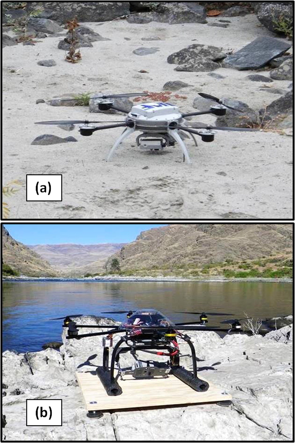
From 2012 to 2014 UASs were tested for counting redds constructed by Chinook salmon below the surface waters of two spawning areas located along a stretch (≈161 km) of a large river. The goal was to increase the understanding of how trends in annual total redd counts could be monitored with less dependence on manned aircraft. The objectives of this paper are (1) to describe 3 years of experience with commercially available UASs and (2) to compare two survey sampling methods for estimating (95% CI) annual total redd counts within each spawning area.

Methods

Study area

The tests were conducted in the portion of the Lower Snake River that flows along the borders of Washington, Oregon, and Idaho, USA, from the Hells Canyon Dam (river km (rkm) 398.7; mouth = 0) to rkm 238.1 located ≈4.0 km upstream from slack water formed by a downstream dam (Fig. 1). This portion of the Lower Snake River is remote and flows through the rugged terrain of Hells Canyon. The Upper Hells Canyon spawning area was one of the test locations, and it begins at Hells Canyon Dam and extends 95.8 km downstream to the Salmon River confluence at rkm 302.9 (Fig. 1). The average width of the Upper Hells Canyon spawning area is ≈84 m and the banks are generally quite steep consisting of bedrock cliffs and large boulder substrate. There are several small sandy beaches and gravel/cobble bars, however. The Lower Hells Canyon spawning area was also studied, and it is generally wider than the Upper Hells Canyon spawning area. The Lower Hells Canyon spawning area extends 64.9 km downstream from the Salmon River mouth to rkm 238.0 where the river transitions into a slack-water reservoir where the fish do not spawn (Fig. 1).
Fig. 1.
Fig. 1. Spawning site locations within the Upper and Lower Hells Canyon spawning areas along the Lower Snake River (map courtesy of Chris Huck of the Idaho Power Company; inset courtesy of the Michigan State University Map Library, Data Source ESR1).
A total of 133 and 94 known shallow-water sites (≤3 m deep) used by Chinook salmon (Fig. 1) that spawn during a 7 week period between 14 October and 7 December have been identified in the Upper and Lower Hells Canyon spawning areas, respectively (Groves et al. 2013). No other fishes construct redds in the two spawning areas during that 7 week period. The number of new sites selected by spawners diminished sharply with increases in spawner escapement between 1994 and 2012 (Groves et al. 2013). Further, the relation between spawner escapement and the number of sites used took the form of a Beverton-Holt stock-recruitment curve (r 2 = 0.92; N = 19 years; P < 0.0001; Groves et al. 2013). Groves et al. (2013) concluded that spawners had identified and used most of the available sites; thus, the probability of identifying a large number of new spawning sites in the future was low.

UASs

The tests in 2012 and 2013 were conducted with an Aeryon Scout™ aircraft (Fig. 2a; overall diameter 0.80 m; height 0.3 m; weight with camera ≈1400 g). The tests were conducted in 2014 with a Mikrokopter hexacopter (Fig. 2b; overall diameter ≈0.7 m; height 0.3 m; weight with camera ≈2200 g). The central hub (fuselage) of each aircraft contained flight and navigation control, onboard GPS, flight recording, multi-axis accelerometers for auto-stabilization, and remote control radio receivers. To maintain consistency between the two aircraft and to increase video resolution, both were mounted with a GoPro model 3+™ video camera. Both aircrafts were powered with a lightweight lithium-polymer battery that provided a total flight time (with camera payload) of ≈20 min.
Fig. 2.
Fig. 2. The Aeryon Scout™ (a) and Mikrokopter hexacopter (b) aircraft used during the 2012–2014 tests conducted along the Upper and Lower Hells Canyon spawning areas.
Ground control stations were provided with each UAS and consisted of a hand-held transmitter and a laptop computer installed with ground-station software that controls the aircraft. This software was used to prepare geo-referenced site maps that were stored within the ground control station. Flight parameters (i.e., the flight plan) for sites sampled within each spawning area were pre-planned and saved, and included defined transects, set waypoints, altitudes, and speed over the ground. Being able to create, store, and upload waypoint files ensured that the aircraft could fly each survey site autonomously in the same manner each year, but manual remote control was always an option. Waypoints were sometimes added, deleted, or changed during flight. Real-time video images were available for viewing on the laptop screen, and video files were also saved on the computer hard drive.

Proof of concept

Pre-deployment

It was necessary to apply for and obtain a Certificate of Waiver and Authorization (COA) from the Federal Aviation Administration (FAA) before using the UASs to count redds. The outcomes of that process are described in the results.
It was not possible to survey all 227 sites with one flight crew because the study area was large and time limited. Survey sampling methods that varied by year were used to randomly select sites to survey (hereafter, survey sites; Table 1). Each survey site was scheduled for survey once a week during the 7 week spawning period. The survey failure rate was calculated as the number of site surveys missed due to technical issues with the UASs or inclement weather divided by the total number of site surveys scheduled.
Table 1.
Table 1. Information describing UAS application to count fall Chinook salmon redds along the Upper and Lower Hells Canyon spawning areas during tests conducted during 2012–2014.
Site surveys
YearSites selectedScheduledCompletedFailure rate (%)Take offsLandingsIncidents
Upper Hells Canyon
2012171199024.458580
2013312172103.21001000
201428196a1903.11011010
Lower Hells Canyon
20122819611342.366660
2013402802597.51291281
20141391a901.164640
Total15710999525185171
a
Does not include sites scheduled to be surveyed the sixth and seventh weeks of the spawning period that were voluntarily not surveyed due to the reversal of Pirker vs. Huerta, Docket CP-217.
After selecting survey sites, flight plans were developed and saved to the ground control station. Although the battery life of the UASs was 20 min, ≈10 min flight plans were developed to ensure an adequate safety margin. Although strict time records were not maintained in all cases, the number of hours required for the pre-deployment activities, deployment, remote data collection, retrieval, post-deployment, and data-processing activities were generally accounted.

Deployment

A jet boat operated by an experienced captain was primarily used to navigate between survey sites, but in some cases, the UAS crew traveled by automobile along a road that ran along the lower 34 km of the Lower Hells Canyon spawning area. When the crew arrived at a survey site for the first time in a given year, the safest point for take-off and landing was located. A 65 cm long, 65 cm wide, and 1 cm thick wooden launch pad was placed flat and level on the ground and a pre-flight check list was reviewed.

Remote data collection

Just prior to take-off, an observer scanned the airspace for manned aircraft, the river for boats, and the surrounding terrain for people. It is important to note that the observer’s duty was not to watch the aircraft, but to maintain surveillance of the surrounding area, and to help determine if the flight operations remained safe with respect to potential air and ground traffic. When all was clear, the operator manually increased the rotor speed until the aircraft lifted off and flew to the survey altitude of 40 m above the river surface. The operator then directed the aircraft to fly autonomously according to the flight plan. While the aircraft was autonomously collecting video footage, the operator and observer could view the real-time location of the aircraft on the geo-referenced site map, the live video feed, and inflight parameters via wireless communication.

Retrieval and post-deployment

The aircraft returned autonomously to its launch point after completing the flight plan and was retrieved either by landing or catching the landing legs of the unit by hand. The aircraft was again checked for physical and mechanical damage, telemetry data were recorded in the flight log book, and captured video was transferred and saved onto a portable storage device.

Data processing

Two biologists processed the recorded video footage after the surveys were completed. One of the biologists had both counted redds from the helicopter (described below) and operated the UAS, whereas the second only assisted during the operation of the UAS. The video footage was reviewed on a large-screen monitor in a darkened room. If needed, contrast, brightness, and colors were adjusted to more clearly define the redds (Figs. 3a, 3b). When necessary, video footage from the same survey site from sequential flights was viewed simultaneously, side by side, to ascertain weekly changes in the patterns of redd location and individual redd size (Figs. 3c, 3d). Such sequential viewing was helpful when one newly constructed redd overlapped with one or more previously constructed redds and the gravel disturbance became a large, contiguous cluster (a.k.a., superimposition; Figs. 3b, 3d). The processed data for each survey site included the number of new redds counted by week, total number of unique redds counted by week, and the grand total number of unique redds counted.
Fig. 3.
Fig. 3. Still shots taken from the UAS video footage collected at a spawning site along the Lower Snake River on 29 October 2012, showing the first redds counted (a), the same spawning site with redds on 5 November 2012 (b), the process of counting the redds on 29 October (c; white ovals), and the process of distinguishing the new redds constructed between the two surveys (black ovals) some of which overlapped with each other and previously constructed redds (d).

Cost comparison

To provide complete coverage of the redd construction period, it was determined that four weekly UAS applications could be temporally spaced across the 7 week spawning season and a total of 50 sites could be surveyed. The cost of all aspects of such an application was projected based on costs observed during the tests. Costs of all aspects of complete census counts made from a manned helicopter each of the 4 weeks were also projected for comparison.

Relative accuracy of manned helicopter surveys

Four manned helicopter surveys were conducted that covered the entire lengths of both spawning areas and spanned the 7 week spawning season during each of the 3 test years (see Groves et al. 2013). A redd count data set was compiled from sites surveyed concurrently with a UAS and from the helicopter (hereafter, index site surveys). Groves et al. (2013) provided evidence for inaccuracy in redd counts made from the helicopter at the higher spawner escapement levels observed during the tests. To evaluate the relative accuracy of the redd counts made from the helicopter, the redd counts from the UAS video footage were treated as the “true” counts, and the relative accuracy of the counts made from the helicopter was calculated as
ReddsHelicopter/ReddsUAS×100
(1)
where ReddsHelicopter was the sum of the number of unique redds counted across the index site surveys from the helicopter for a given spawning area and year, and ReddsUAS was the sum of the number of unique redds counted across the index site surveys from the UAS video footage for the same spawning area and year.

Evaluating two survey sampling methods for estimating (95% CI) annual total redd counts

Although annual census counts of redds had been made from a manned helicopter, and redds at selected sites had been counted with a UAS, the UAS applications did not span the entire spawning period during 2012–2014. Thus, simulation analyses were conducted with existing redd count data collected from a manned helicopter along the entire lengths of the Upper and Lower Hells Canyon spawning areas in 2008–2014. Detailed data collected by the authors (see Groves et al. 2013) were used in the simulation analyses assuming the redd counts were made without error and were the true redd counts. The two methods described hereafter were used to estimate annual total redd counts from a sample of spawning sites drawn from the 2008–2014 redd count data.
Stratified random sampling (STRS) and sampling proportional to size (PPS) methods were compared for estimating (95% CI) annual total redd counts (Scheaffer et al. 1996). The two spawning areas were composed of the primary strata that were further stratified based on historical site use as follows. The average number of redds counted at each spawning site within each spawning area in 2008–2014 were taken from the simulation data set and used to place the sites into five usage categories (average annual redd counts of <1.0, 1.0–9.9, 10.0–19.9, 20.0–29.9, >30.0). It was determined that a maximum of 25 sites per spawning area could be surveyed by a single crew with a UAS during each of four biweekly periods that would span the spawning season.
For STRS, Neyman allocation (Scheaffer et al. 1996) was used to determine how to allocate the 25 sites to be surveyed among the five usage site categories within each spawning area. Neyman allocation uses the variances within each stratum; consequently strata with high variance require more survey effort due to the uncertainty associated with high variance and strata with low variances require less survey effort (Scheaffer et al. 1996). A total of 25 sites for the survey simulations were randomly drawn from the simulation data set with replacement 1000 times to make 1000 redd count estimates for each spawning area and year. Although the redd counts at each of the 25 sampled sites were based on the actual number counted, they were treated as if they were counted from UAS video footage. This was done because, in the future, UAS video footage would provide the number of new redds counted biweekly which would then be summed to calculate the annual total redd count for each of the selected sites.
The PPS method uses a covariate to assign sampling probabilities proportional to the size of each site that were then used to calculate weights for estimating annual total redd counts. The PPS method had the potential to provide 95% CIs on the annual total redd count estimates that were more conservative (i.e., opposed to permissive) with regard to actual coverage and be more efficient (require a smaller sample size) compared to STRS. The PPS method relies on information from previous years to assign weights to more recent years. The weights were based on the prior 4 years redd occupancy data resulting in the sites with higher annual occupancy having assigned higher weights. As such, estimates of total redd counts could only be made for the 5 year period from 2010 to 2014. To facilitate direct comparison between the two sampling methods, the STRS results were restricted to those 5 years as well. The R (R Core Team (RCT) 2015) function PPSS from the package PPS (Gambino 2012) was used to draw 25 sites from each spawning area in the simulation data set with replacement. This was done 1000 times to produce 1000 redd count estimates for each spawning area and year. The Hansen–Hurwitz estimator (Hansen and Hurwitz 1943) was used to find the point estimate and its variance.
To evaluate accuracy of the estimates of annual total redd counts made with STRS and PPS, bias was calculated as both a ratio and a difference. The bias ratio was calculated as the median from each set of 1000 estimates, divided by the corresponding observed annual total redd count. Accuracy declined as the departure of that ratio from 1.0 became greater. To examine the bias and bias distributions in absolute terms, the observed annual total count for a given year and spawning area was subtracted from each of the 1000 estimates of annual total redd counts for that year and spawning area. Then, the medians and the 2.5th and 97.5th percentiles were taken from those 1000 differences and plotted. The 95% CI coverage was compared between the two methods as well. Coverage was calculated for each set of 1000 estimates by determining the percentage of those estimates that contained the corresponding observed annual redd count. Coverage should be approximately 95% if the method is performing as expected.

Results

Proof of concept

The FAA did not issue COAs for commercial purposes in 2012 and 2013. The tests fell under the commercial purposes category because they were funded and conducted by employees of a private company (i.e., Idaho Power Company). The process for obtaining a COA by federal and public entities that had never possessed a COA was difficult to understand and under revision. As such, it was not practical for the staff of US Fish and Wildlife Service or University of Idaho to pursue a COA. The solution in 2012 and 2013 was to contract a public organization that had been granted previous COAs (University of Alaska, Fairbanks, Alaska, USA; 2012-WSA-103-COA). During the 2014 survey season, a court decision (Pirker vs. Huerta, Docket CP-217) reduced the authority of the FAA to regulate the commercial application of UASs. Because of that court decision, the Idaho Power Company biologists were able to conduct the 2014 survey flights without a COA. That case was overturned during the fifth week of the 2014 surveys. The UAS flights were voluntarily discontinued, and the site surveys scheduled for the sixth and seventh weeks of the 2014 spawning period were not conducted.
The number of sites selected for survey, and the number of scheduled site surveys, varied by spawning area and year (Table 1). The survey failure rate declined markedly from 2012 to 2013, and then again from 2013 to 2014 (Table 1). The survey failure rate in 2012 was high because the aircraft malfunctioned possibly due to extensive use over saltwater earlier in the year, and a backup aircraft was not on hand. Thus, site surveys were missed while waiting for backup aircraft to be shipped. In 2013, a backup aircraft was on hand. The 2013 failure rate was influenced partly by human error (e.g., sand in the camera lens, failure to turn the camera on, and lost or copied over data files), but mostly by high rainfall that increased turbidity and made it difficult to view the river bottom. Wind speeds exceeding ≈55 km/h prevented the completion of six and one scheduled site surveys in 2014 within the Upper and Lower Hells Canyon spawning areas, respectively (Table 1).
Over the 3 years of testing, a grand total of 518 take offs and 517 successful landings were made (Table 1). The take offs and landings during the 3 test years were accomplished on a variety of rugged terrains. No problems related to power were experienced with one exception that resulted in an unplanned flight termination in 2013 (i.e., the one missed landing; Table 1). That incident resulted from a poorly secured battery that was jettisoned early in the flight. The aircraft fell into the river near the shore. The backup aircraft was used for site surveys until the downed aircraft was dried and flightworthy. During all other completed site surveys, the aircraft flew well and recorded clear video footage even when wind gusts estimated from the telemetry output data from the ground control station reached ≈55 km/h.
It took an average (±SD; N = 3) of 251 ± 21 h to complete an entire UAS application from pre-planning through data processing during 2012–2014 (Table 2). During each season, on average, time spent in the field was the most time-consuming activity (139 ± 21 h), followed by data processing (80 h or 2 full weeks each year), and pre-deployment planning (32 h each year). When in the field, it took about the same amount of time on average to deploy, remotely collect data, and retrieve the aircraft (68 ± 17 h) as it did to travel among survey sites (71 ± 11 h). At a finer scale, it took an average of 0.5 ± 0.1 h of field time expended to complete data collection at a single site including deployment, actual flight, and travel to the next site with an average of 0.9 ± 0.2 h to complete an entire site survey including pre-planning, field, and post-processing time.
Table 2.
Table 2. Duration in hours of various stages of UAS application to count fall Chinook salmon redds throughout the Upper and Lower Hells Canyon spawning areas combined during tests conducted from 2012 to 2014.
Field
YearPre-deployment planningDRRaTravelTotalPer site surveybData processingTotalTotal per site surveyc
20123249791280.6802401.2
20133290781680.4802800.6
20143265551200.4802320.8
Mean ± SD32 ± 068 ± 1771 ± 11139 ± 210.5 ± 0.180 ± 0251 ± 210.9 ± 0.2
a
Equipment deployment, remote data collection, and equipment retrieval.
b
The annual total number of field hours given divided by the annual total number of successful site surveys from Table 1.
c
The sum of the annual total field and data processing hours given divided by the annual total number of successful site surveys from Table 1.
The total cost of an annual river-wide census count from a manned helicopter was 83% of the total cost of a UAS application (helicopter total cost divided by UAS total cost; Table 3). Greater costs were observed for the UAS application for six of the nine line items because it took longer to prepare for, more time to conduct in the field, required a boat, and required more post-processing time in the office compared to census counts made from a manned helicopter. The aircraft cost line item was much higher for the helicopter because the purchase price of the UAS was amortized.
Table 3.
Table 3. A comparison of the projected total number of hours and costs (Canadian dollars) required to count redds at 50 spawning sites for four weeks of the seven week spawning period with a UAS and four weekly helicopter flights that would provide a complete census of the redds constructed.
Hours per biologistCost
Line itemBiologistsUASHelicopterDifferenceUASHelicopterDifference
Pre-deployment132a8242 1065261 580
Travel to fieldb28801 0531 0530
Field time280c324810 5284 2116 317
Airfared23 6853 6850
Lodginge23 7901 2632 527
Per diemf21 8956321 263
Aircraftg4 21121 056−16 845
Boath5 52705 527
Post-processing257i8497 5011 0536 448
Total322j104j218j40 29633 4796 817
a
From Table 2.
b
From Boise Idaho to Lewiston Idaho.
c
50 sites multiplied by 4 surveys per site multiplied by the average field time per site survey for 2014 (0.4 h) from Table 2.
d
Eight round trip tickets at $461 each.
e
$158 per night per biologist, 12 nights for UAS, and four nights for helicopter flights.
f
$79 per day per biologist, 12 days for UAS, and 4 days for helicopter.
g
$10 528 for each of two UAS amortized over 5 years, $1316 per hour for helicopter flights.
h
$1382 per week including captain wages.
i
200 site surveys (50 sites multiplied by 4 weeks) multiplied by 17 min per site survey (observed for 2014).
j
The number of hours for a given line item multiplied by the number of biologists for that line item summed across line items.
The annual total redd counts taken from the UAS video footage were consistently higher than the corresponding counts made by a biologist from the helicopter during the index site surveys (Table 4). Despite improved accuracy, however, estimates of total annual redd counts made using the UAS count data from the subset of surveyed sites within the two spawning areas in any test year would carry greater uncertainty because the UAS applications did not span the 7 week spawning period. The following analyses evaluated relative accuracy, bias, and coverage of simulated UAS applications that spanned the full spawning period.
Table 4.
Table 4. The relative accuracy (%; eq. (1)) of the manned helicopter surveys by spawning area and year, 2012–2014.
Upper Hells CanyonLower Hells Canyon
YearNReddsHelicopterReddsUASRelative Accuracy (%)NReddsHelicopterReddsUASRelative Accuracy (%)
20121142445992.46101566.7
2013826829491.233776110270.4
2014610618357.91640950381.3
Mean ± SD80.5 ± 19.572.8 ± 7.6

Note: N is the number of index site surveys; ReddsHelicopter is the sum of the number of unique redds counted across the index surveys from the helicopter; and ReddsUAS is the sum of the number of unique redds counted across the index surveys from the UAS video footage.

Evaluating STRS and PPS for estimating (95% CI) annual total redd counts

Accuracy of the annual total redd count estimates made for both spawning areas with STRS was relatively high (>0.98), whereas accuracy of the estimates made with the PPS model was notably lower in several years (Table 5). Large differences were observed in the accuracy of the two methods in 2012 for the Upper Hells Canyon spawning area, and in 2011, 2012, and 2014 for the Lower Hells Canyon spawning area.
Table 5.
Table 5. Results from the 2010–2014 simulation analyses conducted with the STRS and PPS methods (1000 iterations per method by year and spawning area).
STRSPPS
YearObsMedianAccuracyBiasCoverageMedianAccuracyBiasCoverage
Upper Hells Canyon
2010107010670.997−390.610660.996−4100.0
20118748700.995−492.08781.0054100.0
2012101110060.995−594.59260.916−8586.0
2013122012211.001191.212331.01113100.0
2014111911090.991−1093.510960.979−23100.0
Lower Hells Canyon
20108218070.983−1473.68140.991−7100.0
2011107510710.996−487.68760.815−19974.4
20123643570.981−777.23300.907−34100.0
20138518430.991−884.38420.989−9100.0
20148378250.986−1280.37610.909−7675.9

Note: The results include the observed annual total redd counts from the simulation data set (obs); medians of the annual total redd count estimates; those medians divided by the observed counts (accuracy); the difference between the observed counts and those medians (bias, also plotted in Fig. 4); and the percentage of times the 95% CI of a given set of 1000 annual total redd count estimates contained the observed annual total redd count (coverage).

The STRS estimates of annual total redd counts tended to be unbiased in all years (Table 5) and the distribution of error generally symmetric around zero (see the error bars in Fig. 4). The PPS estimates exhibited detectable bias for the Upper Hells Canyon spawning area in 2012, and for the Lower Hells Canyon spawning area in 2011, 2012, and 2014 (Table 5; Fig. 4). With the exception of 2010, the bias distributions for the PPS estimates were positively skewed (see error bars in Fig. 4). Further characterization of the distribution revealed that PPS, as implemented in the simulations, did not produce approximately normal sampling distributions for either spawning area. In fact, neither method produced approximately normal distributions for the Lower Hells Canyon spawning area. In contrast, STRS produced approximately normal sampling distributions for the Upper Hells Canyon spawning area.
Fig. 4.
Fig. 4. Bias distributions (medians close to 0 indicate an unbiased estimate) for STRS and PPS by year and spawning area (Upper Hells Canyon, a; Lower Hells Canyon, b) including the median (STRS black circles; PPS open circles), and the 2.5th and 97.5th percentiles (the lower and top ends of each vertical line) of the 1000 simulated estimates, 2010–2014.
Coverage of the annual total redd count estimates made with STRS and PPS differed dramatically. Coverage probability for the STRS 95% CIs never equaled or exceeded the 95% benchmark in either spawning area, whereas the PPS coverage probability was 100% during 4 of 5 simulation years for the Upper Hells Canyon spawning area, and in 3 of 5 simulation years for the Lower Hells Canyon spawning area (Table 5). In the 3 years when coverage probability was not 100% for PPS, it was quite low reaching levels of only 86%, 74.4%, and 75.9%. Coverage probability tended to be higher for PPS compared to STRS because the PPS 95% CIs were wider than the STRS 95% CIs (Fig. 5).
Fig. 5.
Fig. 5. The median widths of the 95% CIs and the 2.5th and 97.5th percentiles (the lower and top ends of each vertical line) from the 1000 simulated estimates of annual total redd counts made with STRS (black circles) and PPS (open circles) by year and spawning area (Upper Hells Canyon, a; Lower Hells Canyon, b), 2010–2014.

Discussion

Application of UASs provided high-quality video images of redds excavated up to 3 m below the water surface at selected sites, and the redd counts taken from those images were more accurate than counts made from a manned helicopter. The large body of wildlife literature reviewed by Linchant et al. (2015) showed that counts made with a UAS are not always more accurate than counts made by other means (e.g., ground counts) as there was large variation in the accuracy comparisons reported. With regard to fish, Kudo et al. (2012) used a UAS to count Chum salmon about once a week for 8 weeks and also seined and counted the fish weekly from the study area for comparison. The UAS count was lower than the seine count during 7 of the 8 weeks, but higher during 1 week. The total UAS and seine counts were 705 and 1348, respectively. One reason for increased accuracy when counting redds along the Lower Snake River was that the UAS video images were reviewed multiple times, and the between-survey comparisons made it easier to identify new redds through time. Also, observers in the helicopter only had one or two chances to count redds as quickly as possible with no opportunity for later review. As such, counting from the helicopter became increasingly difficult and counts more uncertain as redds became superimposed under high spawner densities. Additionally, the census counts made from the helicopter on a particular day were made by a single observer and not replicated by a second observer. The lack of replicated counts made it impossible to describe the uncertainty (e.g., a 95% CI) in the census counts.
It must be noted that collecting accurate count data at the site level with a UAS was a learning process that required ample funding including the provision of a backup aircraft. The annual cost of UAS application exceeded the annual cost of a manned helicopter survey by $6817, but that cost differential cannot be applied across all studies. As a case in point, the estimated cost of counting Chum salmon within a small study area from a helicopter was about seven times higher than the cost observed for UAS application (Kudo et al. 2012). Collecting data with a UAS also required federal authorization that was very difficult to understand and obtain during the 2012–2014 test years. Obtaining federal authorization has been recognized internationally as one of the major factors impeding the use of UAS technology for natural resource purposes, but there is some evidence that such authorization will become easier to obtain (Linchant et al. 2015). In fact, the FAA granted the Idaho Power Company a COA in 2015.
Another noteworthy point that requires recognition is that the collection of accurate count data at the site level is just one of two important components of enumerating natural resources with UAS technology. Jones et al. (2006), who conducted one of the earliest proof-of-concept tests, stressed the importance of pairing data collected with a UAS with appropriate statistical methods. Efforts to pair accurate count data collected with an unmanned aircraft with statistical methods are undoubtedly increasing, but the peer-reviewed literature on the topic is presently sparse (Linchant et al. 2015). Kudo et al. (2012) regressed weekly UAS counts of Chum salmon against the corresponding weekly seine counts. The two sets of weekly counts were highly correlated (r 2 = 0.93; P < 0.0001), and it was concluded that future abundance estimates could be made by inputting UAS count data into the regression equation. Density estimates made with the Jolly method for elephant (Loxodonta africana) in Africa were potentially biased because it was determined that single observers missed 14.7% of the elephants in the video images (Vermeulen et al. 2013). Undercounting was eliminated by assigning two observers to count the animals. Density estimates made with a generalized linear model for cattle (Bos taurus) in Spain were consistently higher than the known densities (Mulero-Pázmány et al. 2015). The researchers concluded that the bias resulted from focusing the UAS application on areas with high cattle densities and recommended STRS as a remedy.
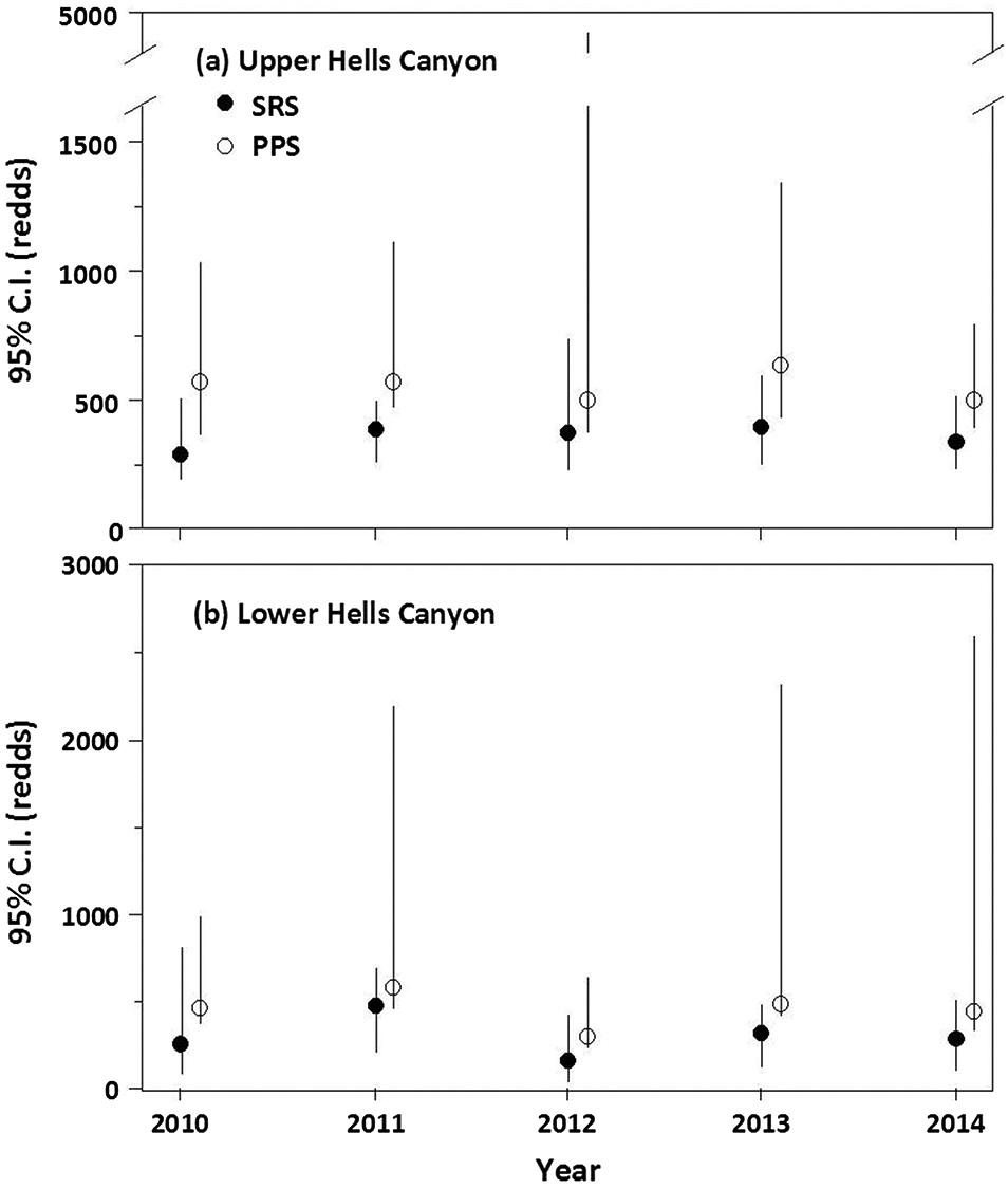
In the simulations conducted to evaluate pairing UAS application with a survey sampling method, STRS provided estimates of annual total redd counts that were more accurate than the estimates provided by PPS. The large majority of the accuracy ratios for STRS were close to 1.000 in Table 5 suggesting a high level of accuracy. Conversely, the relative accuracies reported in Table 4 (converted to proportions) for the site-specific redd counts made from a manned helicopter ranged from 0.579 to 0.924. Comparing those two sets of results at face value provides evidence for the following conclusion. Application of a UAS with STRS would produce estimates of annual total redd counts that would be more accurate than census counts made from a manned helicopter. It is import to recognize, however, that each of the 1000 sets of estimates from simulation analyses also had unreported estimates representing the 2.5th, 25th, 75th, and 97.5th percentiles that would be lower or higher than the median estimate analyzed to calculate the accuracy ratios in Table 5. Thus, in actual field application, when only a single set of sites would be drawn for survey with a UAS in each of the spawning areas in a given year, and only a single annual total count would be estimated for each of those areas, that estimate could undetectably differ from the true annual total counts. Potential users of UASs should conduct simulation analyses with historical data collected within their study areas to fully evaluate the efficacy of UAS application.
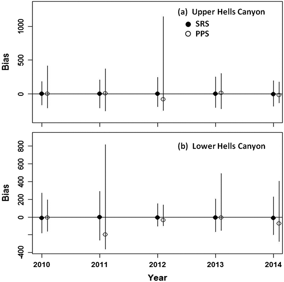
The redd count simulation analyses also detected differences in the coverage of the annual total redd counts estimated with the two survey sampling methods tested. Although STRS produced unbiased estimates, the 95% CIs exhibited under-coverage, notably so for the Lower Hells Canyon spawning area. The performance of PPS was less consistent compared to STRS in both bias and coverage. In years when PPS performed well, it was unbiased and obtained 100% coverage, but that coverage was due to conservative (i.e., wide) CIs. In years when PPS performed poorly, the estimates tended to be biased and the coverage was very low. The relatively poor performance of both methods in the Lower Hells Canyon spawning area corresponded to non-normal sampling distributions in the simulations. The STRS method did achieve a normal sampling distribution for the Upper Hells Canyon spawning area with a sample size of 25 survey sites, whereas PPS did not. Therefore, it is likely that STRS can be used for reliable estimation of total redds in the Upper Hells Canyon spawning area, but a different technique should be explored in the future for the Lower Hells Canyon spawning area.
Wide inter-annual variability in site use by spawners in the Lower Hells Canyon spawning area was likely responsible for both the bias in the PPS estimates and the low coverage of the STRS estimates. For example, a site that was classified as a high-use spawning site based on the historical record of use qualified as a low-use site the year a survey was simulated. One factor that might affect such unpredictable site use is the social aspect of spawning (Groves et al. 2013). If fish begin to spawn at one site earlier than at a second adjacent site, the habitat alterations created by the first spawners might subsequently and disproportionately draw fish to the first site (e.g., for brook trout Salvelinus fontinalis and brown trout Salmo trutta; Essington et al. 1998). In addition to social spawning, covariates that might influence inter-annual variation in spawning site selection include water depth, water velocity, and geomorphology (e.g., Geist and Dauble 1998; Groves and Chandler 1999; Hanrahan 2007). With a covariate that strongly correlated with the redd counts at each site, the PPS method could be modified to produce consistently unbiased, and much more efficient estimates (i.e., require fewer site surveys than needed for STRS). With a more accurate estimation of the variance of use at each site, or a better understanding of the covariates that affect that variance, an appropriate sample size could be obtained to improve the coverage of the annual total redd count estimates made with STRS. However, the sample size of sites to be surveyed could become very large (i.e., approach the point of becoming a census).
Additional survey sampling methods might be considered not only for the Lower Hells Canyon spawning area, but for other large study areas where UAS application is being tested. Adaptive sampling methods are useful for highly aggregated populations (e.g., Woodby 1998; Conroy et al. 2008) as might be the case in the Lower Hells Canyon spawning area. Such adaptive approaches use multiple stages, beginning with either measuring randomly selected sites or performing a low-intensity detection method. Then, sites are added using a selection rule given the data gathered from the first stage. Data are then collected on those additional sites. This process would be repeated until the selection rule results in no new sites (Woodby 1998). Such adaptive approaches may be viable if the extra effort can be allocated during the early portion of a given survey period to develop the sample.

Concluding remarks

Unmanned aircraft paired with survey sampling methods avoid the risk that accompanies manned aircraft flights when enumerating natural resources. The potential for expanding the use of unmanned aircraft is large, especially when the study areas are intermediate or small in size. It is not a simple matter, however, to conclude that coupling the two methods is the best alternative for conducting natural resource surveys in large study areas such as the lower Snake River and its tributaries.
The managers we (i.e., the authors) inform are seeking to recover fall-run Chinook salmon listed under the US Endangered Species Act (National Marine Fisheries Service (NMFS) 1992) that spawn in portions of the Clearwater, Grande Ronde, Salmon, and Imnaha river drainages (Fig. 1) in addition to the Upper and Lower Hells Canyon spawning areas. Manned helicopter flights were replaced with UAS application in Hells Canyon in 2015 for the sake of safety and because the counts made from the helicopter were no longer accurate, whereas the remaining spawning areas continued to be surveyed from a helicopter pending the results of our tests with UAS, and easier access to COAs. Our managers, as well as managers of other large aquatic and terrestrial ecosystems, are now being challenged with a discordant flow of information during a period of transition. Application of UASs will inform management objectives safely but long-term, system-wide census counts will be replaced by estimates with inherent uncertainty. Ongoing manned aircraft surveys will inform those same objectives with risk, while maintaining long-term census counts that have become inaccurate as spawner densities have increased, and do not include estimates of precision.
Use of unmanned aircraft capable of long-range operation beyond line of sight to conduct complete census counts would solve the statistical problem associated with the survey sampling methods described here, but natural resource professionals do not have access to such technology. Furthermore, such operation is heavily restricted in most developed countries (Chabot and Bird 2015). Increasing the number of crews operating UASs within line of sight to achieve a complete census would eliminate problems with bias and coverage. Additional funding, training opportunities to increase the number of certified UAS operators, and streamlined access to COAs would be needed for this solution to work, however. Alternatively, management objectives could be revised with the limitations of UAS application in mind.

Acknowledgements

This paper is dedicated to those natural resource professionals and pilots who have suffered accidents, or who have perished while performing aerial surveys useful for fisheries and other natural resources management. This project could not have moved forward without the staff of the Alaska Center for Unmanned Aircraft Systems Integration of the University of Alaska, Fairbanks who went out of their way to help us after completing their own extensive field seasons. The Idaho Power Company provided the large majority of funding. This research was also supported by Bonneville Power Administration project 199102900. Any use of trade, firm, or product names is for descriptive purposes only and does not imply endorsement by the Idaho Power Company, University of Idaho, or the US Government. No US Endangered Species Permits were required to conduct this research. The findings and conclusions in this article are those of the author(s) and do not necessarily represent the views of the US Fish and Wildlife Service, National Oceanographic and Atmospheric Administration, or the National Marine Fisheries Service.

References

Burner CJ. 1951. Characteristics of spawning nests of Columbia River salmon. US Fish and Wildlife Service Fishery Bulletin, 52: 96–110.
Chabot D, and Bird DM. 2015. Wildlife research and management methods in the 21st century: where do unmanned aircraft fit in? Journal of Unmanned Vehicle Systems, 3: 137–155.
Connor WP, Garcia AP, Connor AH, Garton EO, Groves PA, and Chandler JA. 2001. Estimating the carrying capacity of the Snake River for fall Chinook salmon redds. Northwest Science, 75(4): 363–371.
Conroy MJ, Runge JP, Barker RJ, Schofield MR, and Fonnesbeck CJ. 2008. Efficient estimation of abundance for patchily distributed populations via two-phase, adaptive sampling. Ecology, 89(12): 3362–3370.
Dauble DD, and Watson WG. 1997. Status of fall Chinook salmon populations in the mid-Columbia River, 1948–1992. North American Journal of Fisheries Management, 17(2): 283–300.
Essington TE, Sorensen PW, and Paron DG. 1998. High rate of redd superimposition by brook trout (Salvelinus fontinalis) and brown trout (Salmo trutta) in a Minnesota stream cannot be explained by habitat availability alone. Canadian Journal of Fisheries and Aquatic Sciences, 55(10): 2310–2316.
Gallagher SP, Hahn PKJ, and Johnson DH. 2007. Redd counts. In Salmonid field protocols handbook. Edited by DH Johnson, BM Shrier, JS O’Neal, JA Knutzen, X Augerot, TA O’Neil, and TN Pearsons. American Fisheries Society, Bethesda, Maryland. pp. 197–234.
Gambino J. 2012. Functions for PPS sampling. R package version 0.94 [online]. Available from https://CRAN.R-project.org/package=pps.
Geist DR, and Dauble DD. 1998. Redd site selection and spawning habitat use by fall Chinook salmon: the importance of geomorphic features in large rivers. Environmental Management, 22(5): 655–669.
Groves PA, and Chandler JA. 1999. Spawning habitat used by fall Chinook salmon in the Snake River. North American Journal of Fisheries Management, 19(4): 912–922.
Groves PA, Chandler JA, Alcorn B, Richter TJ, Connor WP, Garcia AP, and Bradbury SM. 2013. Evaluating salmon spawning habitat capacity using redd survey data. North American Journal of Fisheries Management, 33(4): 707–716.
Hanrahan TP. 2007. Bedform morphology of salmon spawning areas in a large gravel-bed river. Geomorphology, 86(3): 529–536.
Hansen MH, and Hurwitz WN. 1943. On the theory of sampling from finite populations. The Annals of Mathematical Statistics, 14(4): 333–362.
Jones GP, Pearlstine LG, and Percival HF. 2006. An assessment of small unmanned aerial vehicles for wildlife research. Wildlife Society Bulletin, 34(3): 750–758.
Kudo H, Koshino Y, Eto A, Ichimura M, and Kaeriyama M. 2012. Cost-effective accurate estimates of adult chum salmon, Oncorhynchus keta, abundance in a Japanese river using a radio-controlled helicopter. Fisheries Research, 119–120: 94–98.
Linchant J, Lisein J, Semeki J, Lejeune P, and Vermeulen C. 2015. Are unmanned aircraft systems (UASs) the future of wildlife monitoring? A review of accomplishments and challenges. Mammal Review, 45(4): 239–252.
Mulero-Pázmány M, Barasona JA, Acevedo P, Vicente J, and Negro JJ. 2015. Unmanned aircraft systems complement biologging in spatial ecology studies. Ecology and Evolution, 5(21): 4808–4818.
National Marine Fisheries Service (NMFS). 1992. Endangered and threatened species: threatened status for Snake River spring/summer Chinook salmon, threatened status for fall Chinook salmon. Final Rule. US Federal Register 57:78 (22 April 1992): 14653–14663.
National Transportation Safety Board (NTSB). 2015. Available from http://www.ntsb.gov.
R Core Team (RCT). 2015. R: a language and environment for statistical computing. R Foundation for Statistical Computing, Vienna, Austria [online]. Available from https://www.R-project.org.
Rieman BE, and McIntyre JD. 1996. Spatial and temporal variability in bull trout redd counts. North American Journal of Fisheries Management, 16(1): 132–141.
Scheaffer RL, Mendenhall W III, and Ott RL. 1996. Elementary survey sampling. 5th edition. Duxbury Press, Belmont, California.
Transportation Safety Board of Canada (TSBC). 2015. Available from http://www.bst-tsb.gc.ca.
Vermeulen C, Lejeune P, Lisein J, Sawadogo P, and Bouché P. 2013. Unmanned aerial survey of elephants. PLoS ONE, 8(2): e54700.
Visser R, Dauble DD, and Geist DR. 2002. Use of aerial photography to monitor fall Chinook salmon spawning in the Columbia River. Transactions of the American Fisheries Society, 131(6): 1173–1179.
Whitehead K, Hugenholtz CH, Myshak S, Brown O, LeClair A, Tamminga A, et al. 2014. Remote sensing of the environment with small unmanned aircraft systems (UASs), part 2: scientific and commercial applications. Journal of Unmanned Vehicle Systems, 2(3): 86–102.
Woodby D. 1998. Adaptive cluster sampling: efficiency, fixed sample sizes, and an application to red sea urchins (Strongylocentrotus franciscanus) in southeast Alaska. In Proceedings of the North Pacific Symposium on Invertebrate Sock Assessment and Management. Edited by GS Jamieson, and A Campbell. Canadian Special Publication Fisheries and Aquatic Science, NRC Research Press, Ottawa, Ontario, 125: 15–20.

Information & Authors

Information

Published In

cover image FACETS
FACETS
Volume 1Number 1January 2017
Pages: 187 - 204
Editor: Karen Kidd

History

Received: 2 May 2016
Accepted: 3 August 2016
Version of record online: 9 November 2016

Data Availability Statement

All relevant data are within the paper.

Key Words

  1. small unmanned aircraft
  2. salmon spawning surveys
  3. population estimates

Sections

Subjects

Authors

Affiliations

Phillip A. Groves
Idaho Power Company, 1221 West Idaho Street, Boise, ID 83702, USA
Brad Alcorn
Idaho Power Company, 1221 West Idaho Street, Boise, ID 83702, USA
Michelle M. Wiest
Department of Statistics, University of Idaho, Moscow, ID 83843, USA
Jacek M. Maselko
Department of Statistics, University of Idaho, Moscow, ID 83843, USA
National Marine Fisheries Service, Alaska Fisheries Science Center, Auke Bay Laboratories, 17109 Pt. Lena Loop Rd., Juneau, AK 99801, USA
William P. Connor [email protected]
US Fish and Wildlife Service, Idaho Fish and Wildlife Conservation Office, 276 Dworshak Complex Drive, Orofino, ID 83544, USA

Author Contributions

PAG, MMW, JMM, and WPC conceived and designed the study.
PAG, BA, and WPC performed the experiments/collected the data.
All analyzed and interpreted the data.
All drafted or revised the manuscript.

Competing Interests

The authors have declared that no competing interests exist.

Metrics & Citations

Metrics

Other Metrics

Citations

Cite As

Export Citations

If you have the appropriate software installed, you can download article citation data to the citation manager of your choice. Simply select your manager software from the list below and click Download.

Cited by

1. Anadromous trout from opposite sides of the globe: biology, ocean ecology, and management of anadromous brown and cutthroat trout
2. Using swim‐up traps to assess Arctic charr ( Salvelinus alpinus ) spawning habitat and the phenology and density of emergent fry
3. Remote sensing of salmonid spawning sites in freshwater ecosystems: The potential of low-cost UAV data
4. Identification of salmon redds using RPV ‐based imagery produces comparable estimates to ground counts with high inter‐observer variability
5. Photogrammetric Counts of Pacific Salmon Using Consumer-Grade Unmanned Aerial Vehicles
6. Technoscience and the modernization of freshwater fisheries assessment and management
7. Photogrammetric counts of pacific salmon by means of unmanned aerial vehicles of consumer grade
8. Networked Unmanned Aerial Vehicles for Surveillance and Monitoring: A Survey
9. Revue des applications et de l’utilité des drones en conservation de la faune
10. Investigation of the spawning sockeye salmon in the pool of the Nachikinskoe Lake (South-Western Kamchatka) with the help of a quadcopter in 2018
11. Assessing the viability of small aerial drones to quantify recreational fishers
12. GIS methods for inventory of pacific salmons spawning grounds in the Amur River
13. Assessing the potential for spectrally based remote sensing of salmon spawning locations
14. A framework for using small Unmanned Aircraft Systems (sUASs) and SfM photogrammetry to detect salmonid redds
15. Use of Drones in Fishery Science
16. Drones for Conservation in Protected Areas: Present and Future
17. Upstream Migration and Spawning Success of Chinook Salmon in a Highly Developed, Seasonally Warm River System

View Options

View options

PDF

View PDF

Get Access

Media

Media

Other

Tables

Share Options

Share

Share the article link

Share on social media