A life-table model estimation of the parr capacity of a late 19th century Puget Sound steelhead population
Abstract
An age-structured life-cycle model of steelhead (Oncorhynchus mykiss) for the Stillaguamish River in Puget Sound, Washington, USA, was employed to estimate the number of age-1 steelhead parr that could have produced the estimated adult return of 69 000 in 1895. We then divided the estimated parr numbers by the estimated area of steelhead rearing habitat in the Stillaguamish River basin in 1895 and under current conditions to estimate density of rearing steelhead then and now. Scaled to estimates of total wetted area of tributary and mainstem shallow shoreline habitat, our historic estimates averaged 0.39–0.49 parr·m−2, and ranged from 0.24 to 0.7 parr·m−2. These values are significantly greater than current densities in the Stillaguamish (mainstem average: 0.15 parr·m−2, tributaries: 0.07 parr·m−2), but well within the range of recent estimates of steelhead parr rearing densities in high-quality habitats. Our results indicate that modest improvement in the capacity of mainstem and tributary rearing habitat in Puget Sound rivers will yield large recovery benefits if realized in a large proportion of the area of river basins currently accessible to steelhead.
Introduction
Recovery of species and distinct population segments (DPS) listed as threatened or endangered under the United States Endangered Species Act “is the process by which listed species and their ecosystems are restored and their future is safeguarded to the point that protections under the ESA are no longer needed” (NMFS 2010). For Pacific salmon and steelhead (Oncorhynchus spp.), this is generally thought to require attaining a condition in which the species or DPS has a probability of persisting for the next 100 years of at least 0.95 (McElhany et al. 2000). Setting endangered species recovery goals and objectives requires a systematic and scientifically rigorous assessment of population needs and the ability of the environment to support those needs (Tear et al. 2005; Beechie et al. 2010). This is especially true when habitat loss is a significant contributor to species declines, and recovery plans emphasize habitat restoration as a means to achieving recovery goals (e.g., Beechie et al. 2003). Within a recovery plan, recovery goals may be narrative statements, but habitat restoration objectives must be specific and measureable actions and targets for improving habitat quantity and quality (Tear et al. 2005; Beechie et al. 2013). One example of this type of recovery plan is that of the threatened Puget Sound steelhead (Oncorhynchus mykiss) in Washington, USA, which declined at least, in part, due to loss and impairment of freshwater spawning and rearing habitats (Hard et al. 2007, 2015).
Recovery of Puget Sound steelhead to a condition of de-listing will require, among other objectives, identifying threshold levels of freshwater juvenile rearing capacity necessary to sustain robust population numbers over multiple generations. However, identifying appropriate thresholds for the production of juvenile steelhead in freshwater will be hampered by lack of information about the capacity of freshwater rearing habitat that supported a much larger adult run size than exists today. Gayeski et al. (2011) employed a Bayesian approach to estimate the total adult run size from the available record of commercial catches for each of four large rivers in north Puget Sound, including the Stillaguamish. The estimated run size in the Stillaguamish River in 1895 ranged from 52 000 to 100 000 based on the 5th and 95th percentiles of the posterior distribution of the Bayes estimate, whereas a recent five-year geometric mean number of natural-origin spawners was 327 (Ford 2011, Table 74, page 237). This 100-fold decline far exceeds what might be expected in response to the loss of only 33% of stream habitat accessible to adult steelhead since 1895 (Gayeski et al. 2011) and a loss of 60% of estimated juvenile steelhead rearing habitat area (this study). Hence, it appears that the productivity of the freshwater rearing environment has experienced a decline since 1895 that is considerably out of proportion to the loss of accessible stream habitat area.
The main objective of this paper is to estimate this loss of productivity by estimating the steelhead parr rearing capacity of the Stillaguamish River in 1895 and compare it to the current productivity. Although post-smolt, marine survival of steelhead has also declined significantly during the past 25 years (Friedland et al. 2014), our focus in this paper is on the importance for the recovery of Puget Sound steelhead of attaining greater densities in steelhead parr rearing habitat than that indicated by recent data. We used an age-structured life-cycle model to estimate the number of age 1 steelhead parr that could produce an adult run size of 69 200 (the mode or most probable value of the posterior distribution of run sizes estimated by Gayeski et al. 2011) over a range of plausible parameter values for both freshwater production and marine (smolt-to-adult return) survival. We then divided the number of parr by estimates of the area of steelhead parr rearing habitat available in 1895 to derive estimates of historical steelhead parr rearing densities (parr·m−2). The life-cycle model incorporates density dependence and a realistic, complex adult age structure that is likely to capture the complex spawning structure of steelhead under minimally disturbed conditions. We conclude with a discussion of the relevance of our estimates to the conservation of Puget Sound steelhead.
Materials and methods
Study area
The Stillaguamish River basin is located in the north-central region of Puget Sound in Washington, USA, discharging to Admiralty Inlet approximately 25 miles north of the city of Everett, Washington (Fig. 1). Puget Sound is a fjord system of flooded glacial valleys that acts as a large inland sea in Washington, USA. It is bounded by the Olympic Mountains to the west and the Cascade Mountains to the east covering 648 000 hectares with approximately 4023 km of shoreline. Numerous large (sixth-order and larger) and medium-sized (fourth- and fifth-order) rivers drain to Puget Sound and currently support 32 independent steelhead populations (Myers et al. 2015). The Stillaguamish River basin contains two major branches, the North and South Forks, which both arise on the west slopes of the North Cascade mountain range. Both forks contain spawning and rearing habitat for steelhead and Pacific salmon species over the majority of their lengths. The river basin has a drainage area of 1230 km2 (Myers et al. 2015, Table D-1), which is the size of an average Puget Sound river basin (Roni et al. 2010). The river is typical of most northern Puget Sound rivers in spanning a mixture of hydrologic regimes from lowland rain-dominated regions with historically forested floodplains to transitional rain/snow mixed piedmont, to snow-dominated forested headwaters (Myers et al. 2015). All hydrologic and climatic regions, except for small first- and second-order headwater tributaries provided historical spawning and (or) rearing habitat for steelhead.
Fig. 1.
Life-cycle model
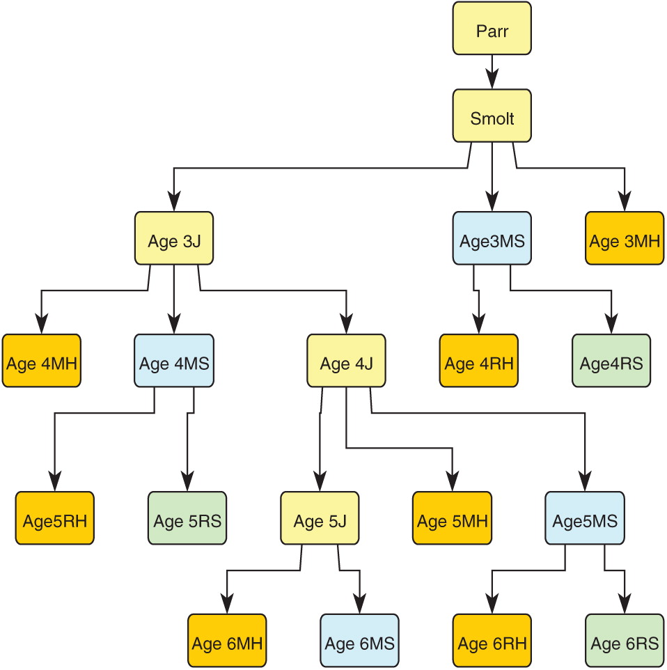
We modeled a steelhead population consisting of a total of six age-classes, with four adult ages (3–6). We modeled females only and assumed a 1:1 sex ratio (Withler 1966; Ward and Slaney 1988; Seamons et al. 2004). The model includes repeat spawning at ages four, five, and six because repeat spawning is believed to have been an important characteristic of steelhead life history prior to the major reductions in winter-run steelhead population sizes during the past 40 years (Hard et al. 2015). The model consists of 19 stages. This results in a square population projection matrix, 19 rows by 19 columns, with fecundity values in the first row and transition rates or zero entries in all other rows. Life stages, transition rates, and fecundities used in the projection matrix and their abbreviations are listed in Supplementary Material 1, Tables S1 and S2. Figure 2 shows a schematic of the life-cycle model starting with parr (age 1) and terminating at each adult age (3–6) and life stage or fate (maiden or repeat spawner, surviving to spawn or harvested).
Fig. 2.
Fecundity (# eggs·female−1) is treated as age- and type-specific (maiden or repeat spawner) based on weight-at-age (Supplementary Material 1, Table S2; Supplementary Material 2). The model includes a single smolt age-class (age 2), which is the most common smolt age for most coastal and Puget Sound steelhead populations (Withler 1966; Quinn 2005; Hard et al. 2015). Population projections of the model were conducted at annual time steps.
Density dependence is incorporated during the period of freshwater residence prior to smolting in the transition from emergent fry-to-age-1 (parr). Accordingly, the model includes two sub-age-1 life stages: eggs and fry. Fry-to-parr survival (fp) is modeled as a type II (Beverton–Holt) function with fixed parameters α and β:where α is the inherent maximum fry-to-parr survival rate at low density under optimal conditions, β is the inverse of the number of fry at which fry-to-adult survival = α/2, and n fry is the number of fry. The number of fry is:where n eggs is the total egg deposition, sr is the sex ratio, ef is the deterministic egg-to-fry survival rate. Consequently, fp will vary nonlinearly with the number of fry produced by each year’s total spawner abundance as will the number of parr produced the following year by each age and type spawner. All other life-stage transitions are considered deterministic and density independent. The model tracks all life stages from egg deposition to adult return by age and stage class, so that production by each spawner type (age and repeat-spawning status) could be accounted separately.
(1)
(2)
For modeling convenience, we assume that repeat spawners attempt to repeat spawn the year after their maiden spawning and that there are no third-time spawners. Repeat spawning the year after maiden spawning was found to be the most common pattern in steelhead in Kamchatka as determined by scale analysis of several hundred samples collected by a joint US-Russian conservation research program between 1996 and 2005 (Pavlov et al. 2001; N. Gayeski, personal observation, 2015). Repeat spawning was modeled for each maiden spawner in age-classes three to five by simply assigning an age-specific probability of surviving spawning to re-enter the ocean. We assumed that there was no difference in reproductive effort between maiden spawners in a given age-class that succeeded in repeat spawning and those that did not. The maximum adult age was set at six and the maturation rate of six-year old fish was set implicitly to 1. Modeling was conducted in MATLAB 7.10.
Puget Sound steelhead in the late 19th century were harvested exclusively in terminal areas (river mouths and associated estuary or nearshore) and in-river fisheries (Wilcox 1898). Thus, only mature fish, both maiden and potential repeat spawners, were harvested. Gayeski et al. (2011) argued that given that the peak commercial harvest of steelhead in Puget Sound occurred in 1895, six years after statehood and the initiation of large-scale commercial fishing for steelhead, the total adult return (harvest plus spawning escapement) was likely recruited from a population at or very near its unfished equilibrium abundance, as determined by the average conditions in freshwater and the marine environment that existed in the final quarter of the century. Gayeski et al. (2011) employed a Bayesian approach to estimate the posterior distribution of the 1895 adult return to the Stillaguamish from the reported commercial steelhead catch for the Stillaguamish augmented by estimates of unreported, non-commercial in-river harvest of steelhead by settlers and others based on historical records and reports. The commercial harvest data were reported in pounds, which Gayeski et al. converted to estimates of total numbers landed using a distribution of average steelhead weights estimated for the period. The total return was then estimated from the estimated total numbers landed and an estimate of the distribution of the total harvest rate assuming a binomial distribution for the harvest process. The posterior mode (single most probable value) of the estimated total adult return in 1895 was 69 200 corresponding to an estimate of 34 600 adult females assuming a sex ratio of 1:1.
Gayeski et al. (2011) estimated that this return was most likely harvested at a rate of nearly 55%, yielding a total harvest of females of nearly 18 900 and a spawning escapement of approximately 15 700. We assumed that this was the case and employed the life-cycle model to estimate the number of age-1 individuals that must have been produced in order to recruit a female population of 34 600. We did this by running the model for 25 time steps (years) starting with 10 years of no harvest and adding harvest at time step 11 that built up steadily to a maximum rate of 0.545 at time step 16 equal to the harvest rate on the 1895 population estimated by Gayeski et al. (2011). The model was run for an additional 9 time steps to verify that the year 16 total catch was a maximum, reflecting the historical harvest record (Fig. 3). The density-dependence capacity parameter was adjusted to achieve the estimated 1895 total catch and total spawner abundance, as described below. The model was then run with the harvest rate set to zero to determine the total unfished equilibrium abundance of all ages at the stable age distribution. We refer to this henceforth as the 1895 equilibrium.
Fig. 3.
We tracked the annual abundance of harvested and unharvested maiden and repeat spawners separately in order to evaluate the impact of harvest on age-classes and on maiden and repeat spawners. The model has 19 stages, including 17 stages for the four oldest age-classes, of which 14 stages are matures. These enable the model to keep track of all spawner life histories and the life histories of all harvested matures (Fig. 2, Table S2).
Fertilities, also referred to as “effective fecundities,” are measured as the number of age-1 progeny (parr) produced by each spawner of a particular age and type, x; that is, the number of offspring surviving to year t + 1 produced by each age-x spawner in year t. These numbers occupy the first row of the square population projection matrix. Thus, the model assumes a prebreeding census, whereby parents are counted each year prior to spawning and their offspring are counted prior to spawning the following year. Fertilities are, therefore, matrix elements generated by underlying vital rates. The vital rates are fecundity (eggs/age and type female), sex ratio, egg-to-emergent fry survival, and density-dependent fry-to-parr survival (Supplementary Material 1, Table S2). Fecundity was treated as age- and size- (weight)-specific for both maiden and repeat spawners in each mature age-class. Since repeat spawners must recover body condition upon re-entering marine waters before they invest energy in gonad production and because they have less time to feed in marine waters before returning to freshwater to spawn than maiden fish of the same age, we assigned repeat spawners a fecundity value slightly greater than maiden spawners in the previous age-class (to account for some body size increase) but less than the value assigned to maiden spawners in the same age-class.
Age-specific weights and fecundities are based on length, weight, and fecundity data collected from steelhead in western Kamchatka on the Russian North Pacific Rim in 2001–2004 (N. Gayeski, personal observation, 2015), and scale analyses of the same individuals made by Dr. Kiril Kuzhichin at the Department of Ichthyology, Moscow (Russia) State University. We used data from Kamchatka because we had fecundity (egg number) and length, weight, and age data for each of approximately 80 individual females. We selected representative lengths-at-age for 3-, 4-, 5-, and 6-year-old maiden and repeat-spawning females that provided representative weights for given lengths and ages. We compared both measured and estimated fecundity-at-length from the Kamchatka data to length-fecundity data for several British Columbia steelhead populations provided to the lead author by Dr. Bruce Ward to evaluate how representative of North American steelhead Kamchatka steelhead are. Kamchatka steelhead had slightly greater fecundity at a given length and weight than the majority of British Columbia winter-run populations. We then adjusted the expected fecundity-at-length downward by adjusting the intercept of the natural log–log regression of fecundity on length of the Kamchatka samples to obtain an average fecundity approximately equal to the mean value reported by Quinn (2005, Table 15-1) that was based on a survey of available published and unpublished data, including the British Columbia data that we examined. We expected that the average fecundity value reported in Quinn (2005) was more likely than the unadjusted Kamchatka data to be representative of Puget Sound steelhead in the late 19th century, as indicated by the range of average steelhead weights reported by Gayeski et al. (2011). The resulting parameterization of the model was corroborated by the model’s achieving the target average adult weight of Puget Sound winter-run steelhead of 8.25 lbs. estimated by Gayeski et al. (2011). Length-weight and length-fecundity equations are provided in Supplementary Material 2. Age-specific fecundities are listed in Supplementary Material 1, Table S2.
Modeling the Stillaguamish circa 1895 steelhead population
Estimating the number of parr produced at the 1895 equilibrium requires that we appropriately partition the recruitment process between the freshwater and marine (post-smolt) periods. Because there are scant empirical data for annual survival rates of smolts and post-smolt age-classes of Pacific salmon and steelhead, we chose two marine survival scenarios, one low and one high, that we believe bracket the likely true values of age-specific post-smolt marine survival of steelhead during the late 1800s.
Modeled marine survival
We started from an estimate of average smolt weight of 54 g, which is equivalent to a smolt fork length of 175 mm and Fulton’s Condition Factor K [W (g) × 100/L (cm)3] of 1.0, and assumed a smolt-to-age-3 survival rate of 0.20 (Ward and Slaney 1988; Quinn 2005). Age 3 is the earliest age of maturation and age 6 the oldest. We estimated the survival rate from age 3 to age 6 for fish that first mature at age 3 to be 0.40 for the low marine survival scenario and 0.80 for the high survival scenario. The value of 0.40 corresponds to an average annual survival rate of 0.74, and the value of 0.80 to an average annual rate of 0.93. We assumed that annual marine survival increases with size, and therefore with age. To determine age-specific annual marine survival values for ages 3, 4, and 5 that reflect this assumption while meeting the cumulative survival constraints of the two survival scenarios, we applied the allometric growth-survival model of McGurk (1996) to the length- and weight-at-age data we chose for the model. The weights-at-age for ages 3–6 were independently constrained by having to achieve an average fish weight of 8.25 pounds, the mean of the weight range estimated by Gayeski et al. (2011), and the total weight of the catch estimated for the Stillaguamish by Gayeski et al. (2011). Having chosen the weights of each spawner age and type (maiden or repeat spawner), we applied the McGurk model to the average weight of smolts and each post-smolt maiden spawner age-class and estimated annual age-specific survivals using parameter values from within the range estimated for steelhead by McGurk (1996). This resulted in values of 0.73, 0.74, and 0.75 for the annual rates of ages 3, 4, and 5 immatures, respectively. Values for the high survival scenario were 0.92, 0.93, and 0.94, respectively.
Modeled maturation and repeat spawning rates
To determine the proportions of spawners of each age and type (maiden and repeat) in the total return, we estimated age-specific maturation rates of ages 3–5 and post-spawning survival rates of maiden spawners ages 3–5 that would result in repeat spawner proportions of returning adults between 20% and 30% (Withler 1966; Pavlov et al. 2001) and would achieve the target average weight of returning adults of 8.25 pounds, assuming that all adult ages and types were equally susceptible to harvest and thus were represented in the total catch in direct proportion to their relative abundance in the total return. We assumed that post-spawning survival increased with the size and age of maiden spawning fish. These values (Sp3S, Sp4S, Sp5S; Supplementary Material 1, Table S2) represent the proportions of maiden spawners at each age that survive to re-enter the ocean at a point in the year at which their survival from that point to the next spawning year is equal to the annual survival rate of immatures of the same age (S34, S45, S56; Supplementary Material 1, Table S2), so that the total survival of repeat spawners to repeat spawning the following year is equal to the product of the two rates (e.g., Sp3S × S34; Supplementary Material 1, Table S2).
Modeled freshwater survival
Given the model values for age-specific fecundity, maturation rates, probabilities of repeat spawning, and marine survival rates, it remained to determine the density-dependent parameters alpha (α) and beta (β) and values for egg-to-fry (ef) and parr-to-smolt (ps) survival. We chose a value of 0.2 for egg-to-fry survival based on a range of literature values (Ward and Slaney 1993; Quinn 2005), taking into consideration that this is an average value for the entire Stillaguamish watershed that spans a range of mainstem and tributary spawning geologies and habitat conditions.
We considered two different values for the density-dependence alpha parameter and for ps, the density-independent parr-to-smolt survival parameter. The alpha parameter is the value for the survival rate of fry to age 1 (parr) when fry densities are very low. We chose values of 0.20 and 0.40. For parr-to-smolt survival, we chose a value of 0.3, the value used by the Puget Sound Steelhead Technical Recovery Team for current optimal conditions (Quinn 2005; Hard et al. 2015, Appendix C), and a value of 0.4 as a conservative estimate for the less anthropogenically disturbed habitat conditions that likely existed throughout the Stillaguamish basin in the late 19th century relative to current conditions. The value of 0.4 is similar to several (Oosterhout et al. 2005; Pess et al. 2011) contemporary estimates of over-winter survival of pre-smolt coho salmon in high-quality habitats. Pre-smolt coho are smaller in body size than steelhead parr and can be expected to survive at lower rates than steelhead parr in similar quality habitats. Given values for all parameters, the total equilibrium abundance is determined by the beta parameter of the density-dependence function, which controls the response of fry-to-parr survival to fry density, and therefore functions as the fry capacity parameter.
Thus, we evaluated juvenile production under four variants of the freshwater component of the life-cycle model corresponding to all combinations of the two parameters governing freshwater survival, α (0.2 or 0.4) and ps (parr-to-smolt, 0.3 or 0.4), for each of the two sets of post-smolt marine survival parameterizations, a total of eight parameterizations of the model. For each of the eight parameterizations, we ran simulations for a period of 25 years under a no harvest and a harvest scenario starting at the unfished equilibrium abundance and stable age distribution. For the harvest scenario, we set the base harvest rate to 0.545, the posterior mode of the estimate in Gayeski et al. (2011). Figure 3 shows the time trajectory for one of the eight parameterizations under the harvest scenario. (Note that since all eight parameterizations of the model are constrained to achieve the same equilibrium total and component adult age and stage (maiden or repeat) abundance, the time trajectories of each are identical to one another within rounding error, except for difference in the proportion of repeat and maiden spawners between the four low and four high marine survival scenarios. Hence only one such trajectory is shown.)
We recorded summary data for equilibrium conditions for each of the eight parameterizations of the model. The value of the density dependence capacity parameter, β, under equilibrium conditions was determined by trial and error by first identifying the stable age distribution of the model and then running the harvest scenario as described above and tuning the beta parameter and the initial population abundance until the total female harvest and spawner escapement corresponded closely to the values estimated by Gayeski et al. (2011) (female spawners = 15 743, total female harvest = 18 857, total female return = 34 600 at simulation year 16 with the harvest rate = 0.545). Equilibrium values of the quantities of interest were then determined by setting the harvest rate to zero.
Results
Figure 4 shows the equilibrium parr abundance for all eight model scenarios, in addition to the mean of the four low and four high scenarios, and the grand mean of all eight scenarios. The model output of all parameters for the most favorable and most unfavorable of the eight survival scenarios (H4 and L1, respectively) together with the averages of the four low and four high marine survival scenarios are listed in Table 1. The complete results for each of the eight models are listed in Supplementary Material 1, Table S3.
Fig. 4.
Table 1.
| Parameters/model | Scenario L1 | Average low | Scenario H4 | Average high |
|---|---|---|---|---|
| Mean fecundity at stable age | 4924 | 4924 | 4832 | 4832 |
| Egg-to-fry | 0.2 | 0.2 | 0.2 | 0.2 |
| Alpha | 0.2 | 0.3 | 0.4 | 0.3 |
| Beta | 1 / 6 383 700 | 1 / 3 861 600 | 1 / 1 090 700 | 1 / 2 036 925 |
| Parr-smolt | 0.3 | 0.35 | 0.4 | 0.4 |
| Smolt-ocean age 3 | 0.2 | 0.2 | 0.2 | 0.2 |
| pMat4 | 0.2636 | 0.2636 | 0.3306 | 0.3306 |
| pMat5 | 0.3648 | 0.3648 | 0.3974 | 0.3974 |
| Ocean age 3-to-ocean age 4 | 0.73 | 0.73 | 0.92 | 0.92 |
| Ocean age 4-to-ocean age 5 | 0.74 | 0.74 | 0.93 | 0.93 |
| Ocean age 5-to-ocean age 6 | 0.75 | 0.75 | 0.94 | 0.94 |
| Female spawners at equilibrium | 39 817 | 39 452 | 40 038 | 40 231 |
| Proportion repeat spawners | 0.235 | 0.235 | 0.286 | 0.286 |
| Fry-parr at equilibrium | 0.049 | 0.043 | 0.021 | 0.025 |
| Total fry | 39 188 957 | 38 830 384 | 38 693 191 | 38 880 379 |
| Total parr | 1 926 005 | 1 670 472 | 825 993 | 968 562 |
| Total smolt | 577 802 | 572 533 | 330 397 | 332 003 |
| Fry-to-smolt | 0.0148 | 0.0148 | 0.0086 | 0.0086 |
| Egg-to-smolt | 0.0030 | 0.0030 | 0.0017 | 0.0017 |
| Cohort smolt-to-adulta | 0.105 | 0.105 | 0.172 | 0.172 |
| Egg-to-adulta | 0.000 311 | 0.000 311 | 0.000 295 | 0.000 295 |
| Spawner-to-spawnera | 1.54 | 1.54 | 1.46 | 1.46 |
| Cohort smolt-to-adultb | 0.138 | 0.138 | 0.237 | 0.237 |
| Egg-to-adultb | 0.000 408 | 0.000 408 | 0.000 406 | 0.000 406 |
| Spawner-to-spawnerb | 2.02 | 2.02 | 2.02 | 2.02 |
a
Cohort smolt-to-adult, egg-to-smolt, and spawner-to-spawner measured for maiden (first-time) spawners only.
b
Cohort smolt-to-adult, egg-to-smolt, and spawner-to-spawner measurements including separate accounting of repeat spawners.
The strongest contrast in the outputs is between the two marine survival scenarios. Density-dependent fry-to-parr survival at the unfished equilibrium is significantly lower under high post-smolt survival (0.021–0.029) than under low post-smolt survival (0.037–0.049). This results from higher values for the fry capacity parameter beta (lower fry capacities) under the high marine survival scenarios and is illustrated in Table 1.
The same number of total fry is produced at equilibrium under all models. The mean number of fry (males and females) across all eight models is 39 000 000 with a coefficient of variation (c.v., standard deviation/mean) of 0.006. Parr and smolt production are more variable. Parr production ranges from a low of 826 000 under model H4 to a high of 1 926 000 under model L1, and smolt production ranges from a low of 330 000 to a high of 578 000. Mean parr production over all models is 1 320 000 with a c.v. of 0.33. Mean smolt production is 452 000 with a c.v. of 0.28. The averages (c.v.) for the four low survival scenarios are 1 670 000 (0.14) and 573 000 (0.005). The averages (c.v.) for the four high survival scenarios are 969 000 (0.14) and 332 000 (0.003).
The proportions of repeat spawners are noticeably greater than for any current Puget Sound steelhead population for which there are data (Hard et al. 2015): 0.235 for the low post-smolt survival scenarios and 0.286 for the high ones. Calculation of cohort smolt-to-adult return and female spawner-to-total adult (males plus females) return values reveals the importance of repeat spawning in the life-cycle model. Calculated only for first-time spawners for the low marine survival scenario, the cohort smolt-to-total adult rate is 0.105 and the female spawner-to-total adult return rate is 1.54 (calculated from mean fecundity and the mean egg-to-adult survival of 0.0003); for the high-survival scenario, the cohort smolt-to-adult rate is 0.172 and the female spawner-to-total adult return rate is 1.46. In other words, the population cannot replace itself at equilibrium (which would require two adults returning for each female spawner).
When cohort and egg-to-adult survival are calculated by including repeat spawners, the cohort smolt-to-total adult return rate for the low post-smolt survival scenario is 0.138 and for the high survival scenario is 0.237. Egg-to-adult survival under both scenarios is 0.0004, an increase of over 30% from the calculation based only on maiden spawners. These raise the female spawner-to-total adult return rate to just over 2.0, assuring replacement at equilibrium.
Juvenile production scaled to historical rearing habitat
The production of parr of both sexes from the eight models ranged from 826 000 to 1 926 000 and averaged 1 320 000 (Table 1; Supplementary Material 1, Table S3). Gayeski et al. (2011) estimated that 668 linear kilometers of mainstem and tributary stream habitat was accessible to winter-run steelhead in the Stillaguamish River in 1895. We updated this estimate using data for historical mainstem and tributary rearing habitat in the Stillaguamish (Pess et al. 1999; Pollock et al. 2004). We estimate that there were a total of 706 km of tributary habitat available for juvenile steelhead rearing and 160 km of mainstem. For tributaries, we estimated the average channel width available to steelhead rearing during near baseflow conditions during the summer and fall growing season to be 3 m based on the two sources cited above, Roni et al. (2010), and unpublished field survey data by two of us (Pess and Beechie). This resulted in an estimated total tributary rearing area of 2 118 000 m2. For mainstem rearing habitats, we used a range of estimates of the average width (each bank) over the total length of mainstem shallow shoreline available for juvenile steelhead rearing during the summer and fall growing season of 2, 3, and 4 m (4, 6, and 8 m both banks combined). The shallow shoreline is defined as the area of mainstem river channel adjacent to the bank where channel depth is no greater than 0.5 m and surface current velocity is not greater than 0.5 m·s−1 (Stanford et al. 2005). This is the area of river main channels where we expect the majority of O. mykiss parr to rear during baseflow and near-baseflow conditions during the summer/fall growing season. This results in a range of total mainstem rearing habitat area of 640 000–1 280 000 m2. Added to the estimate of tributary rearing area, these estimates yield an estimate of total historically available juvenile parr rearing area of 2 780 000, 3 078 000, and 3 398 000 m2 (Table 2).
Table 2.
| Habitat type | Length (km) | Length (m) | Width (m)a | Area (m2) |
|---|---|---|---|---|
| Tributaries | 706 | 706 000 | 3 | 2 118 000 |
| Mainstem 1 | 160 | 160 000 | 4 | 640 000 |
| Mainstem 2 | 160 | 160 000 | 6 | 960 000 |
| Mainstem 3 | 160 | 160 000 | 8 | 1 280 000 |
| Tribs + mainstem 1 | 2 758 000 | |||
| Tribs + mainstem 2 | 3 078 000 | |||
| Tribs + mainstem 3 | 3 398 000 |
a
Tributary width is total width; mainstem width is the total for both banks combined.
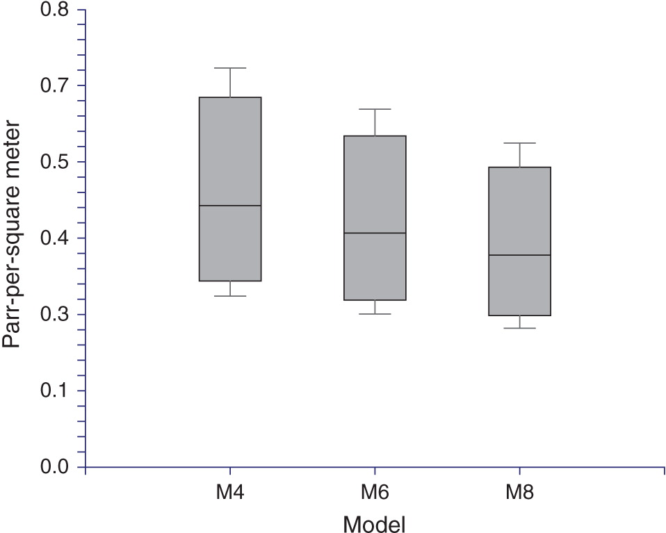
Dividing each of the eight estimates of 1895 equilibrium parr production by the three estimates of total rearing area yields estimates of parr densities in juvenile rearing habitats of 0.24–0.70 parr·m−2. For the average total parr production of 1 320 000 (averaged across all eight model runs), rearing densities range from 0.39 to 0.48 parr·m−2. The average across the four low marine survival scenarios is 0.49–0.61 parr·m−2. The average across the four high marine survival scenarios is 0.29–0.35 parr·m−2 (Table 3).
Table 3.
| Estimated rearing area (m2) | ||||
|---|---|---|---|---|
| Model | Total parr | 2 758 000 | 3 078 000 | 3 398 000 |
| L1 | 1 926 005 | 0.698 | 0.626 | 0.567 |
| L2 | 1 435 288 | 0.520 | 0.466 | 0.422 |
| L3 | 1 900 214 | 0.689 | 0.617 | 0.559 |
| L4 | 1 420 379 | 0.515 | 0.461 | 0.418 |
| H1 | 1 113 266 | 0.404 | 0.362 | 0.328 |
| H2 | 831 380 | 0.301 | 0.270 | 0.245 |
| H3 | 1 103 609 | 0.400 | 0.359 | 0.325 |
| H4 | 825 993 | 0.299 | 0.268 | 0.243 |
| Average of all eight models | 1 319 517 | 0.478 | 0.429 | 0.388 |
| Average of L1:L4 | 1 670 472 | 0.606 | 0.543 | 0.492 |
| Average of H1:H4 | 968 562 | 0.351 | 0.315 | 0.285 |
Figure 5 shows box plots of parr densities for all eight modeled scenarios for each of the three estimates of total rearing area.
Fig. 5.
Parr capacity in the Stillaguamish River under current conditions
Roni et al. (2010) estimated steelhead parr production in a modeled Puget Sound watershed the size of the Stillaguamish before restoration, which is to say, under current conditions. They estimated the lengths of three types of stream habitats, small, medium, and large, and the current number of parr produced by each. Small and medium streams correspond to tributaries in our analysis: large streams to mainstems. The total length of large streams is 117 751 m (118 km). Steelhead parr production in large streams was estimated to be 99 238. Using our estimates of mainstem rearing habitat area as equal to stream length × 4, 6, and 8 m, the estimated rearing areas of large streams are 471 000, 707 000, and 942 000 m2 (Table 4). This yields parr densities of 0.21, 0.14, and 0.11 parr·m−2, respectively. These densities are lower than the mean values of our historic estimates of 0.48, 0.43, and 0.39 parr·m−2, respectively (Table 3).
Table 4.
| Habitat type | Length (m) | Area (m2) |
|---|---|---|
| Tributaries | 184 265 | 552 795 |
| Mainstem 1 | 117 751 | 471 004 |
| Mainstem 2 | 117 751 | 706 506 |
| Mainstem 3 | 117 751 | 942 008 |
| Tributaries + mainstem 1 | 302 016 | 1 023 799 |
| Tributaries + mainstem 2 | 302 016 | 1 259 301 |
| Tributaries + mainstem 3 | 302 016 | 1 494 803 |
Discussion
We provide the first model-based estimate of steelhead parr rearing capacities and associated densities for a representative Puget Sound river basin under conditions that existed in the late 19th century that were considerably less anthropogenically disturbed than today. We employed an age-structured life-cycle model to generate the number of steelhead parr (age-1) produced under equilibrium conditions by a population of female spawners in a representative river basin in Puget Sound under the environmental conditions that existed at the end of the 19th century and that are assumed to have been more favorable to the production of anadromous salmonids than today (Hard et al. 2007, 2015; Myers et al. 2015). The modeled population consisted of an array of sizes, ages, and spawning types (maiden and repeat) in proportions that are likely to have existed at that time given available historical information (as summarized, e.g., in Withler 1966). We parameterized weight- and fecundity-at-age with data from populations in western Kamchatka that still exhibit the complex life histories that likely characterized Puget Sound steelhead populations under the less anthropogenically disturbed conditions of the late 19th century (Pavlov et al. 2001). We corroborated the appropriateness of the parameterizations of weight and fecundity by verifying that the model achieved the average adult weight of 8.25 lbs estimated by Gayeski et al. (2011) for Puget Sound winter-run steelhead in 1895 and an average fecundity of 4900 reported by Quinn (2005).
Age- and stage-structured life-cycle models are appropriate to contexts such as ours where the aim is to examine the relationships between population numbers at different life stages and (or) between one or more critical life stages and candidate environmental covariates affecting growth and survival. Our approach is consistent with other uses of age- and stage-structured life-cycle models employed in various conservation and management contexts involving salmon (Greene and Beechie 2004; Oosterhout et al. 2005; Scheuerell et al. 2006) and marine mammals (Brault and Caswell 1993; Olesiuk 2005). In our case, we sought to improve our understanding of how the complex adult spawning life histories and population abundance that characterized Puget Sound steelhead populations at the end of the 19th century were maintained across generations by modeling the life cycle of a representative Puget Sound steelhead population, the Stillaguamish River population. Specifically, we were interested in characterizing the parr production and associated adult life history required to sustain the 1895 equilibrium abundance, and then comparing that historical parr capacity to potential parr production under current habitat conditions. By modeling the entire life-cycle and making judicious use of available data pertaining to steelhead life history, we were able to achieve those aims.
Changes in marine survival of Puget Sound steelhead since 1895
Marine (smolt-to-adult return) survival rates are known to have declined during the past quarter of a century and have undoubtedly contributed to recent declines and listing of several steelhead populations under the Endangered Species Act, including Puget Sound steelhead (Smith et al. 2000; Ward 2000; Welch et al. 2000; Friedland et al. 2014). Friedland et al. (2014), for example, estimated changes in smolt-to-adult survival rates for steelhead between 1977 and 2005 from the well-studied Keogh River population on the East Coast of Vancouver Island, British Columbia. They estimated that average survival rates decline threefold from 14% during the first half of the period to 5% during the second half. Survival rates of Puget Sound populations over the past decade may have been even lower (Moore et al. 2015).
It may be thought that such changes in marine survival render our estimates of the parr capacity of the Stillaguamish River in 1895 of little relevance for the conservation of Stillaguamish steelhead under current conditions. We do not believe that this is the case. First, our estimates of first year post-smolt survival and age-3-to-age-6 survival to adult return for low and high marine survival scenarios resulted in cohort smolt-to-adult return survival rates of 0.105–0.172 (Table 1). This is comparable to mean survival rates estimated for the Keogh River during the mid-1980s of 0.14–0.16, with survival rates for individual cohorts as high as 0.26 (Ward and Slaney 1988; Friedland et al. 2014). Hence, our modeled marine survival rates are likely conservative with respect to conditions that existed in the late 19th century. Second, the effect of employing conservative estimates of marine survival on our estimates of parr capacity would be to inflate those estimates relative to the number of parr at equilibrium required under more favorable marine survival rates (Table 1; Supplementary Material 1, Table S3). That is, the greater the marine survival, the fewer number of parr and smolts required in order to recruit a given number of spawning adults.
For similar reasons, our acceptance of the best estimate of the 1895 equilibrium of the Stillaguamish River of 69 200 estimated by Gayeski et al. (2011) for the purpose of estimating parr capacity in 1895 is conservative. If the adult estimate is inflated, then our estimate of parr capacity in 1895 will be similarly inflated. If anything, therefore, our estimates of parr capacity and densities in the Stillaguamish in 1895 would push the bounds of realistic parr densities that we estimate were required to sustain the adult equilibrium abundance estimated by Gayeski et al. (2011). As we show in the following section, this does not appear to be the case. This result has the indirect effect of providing independent evidence that the estimate of Gayeski et al. (2011) is biologically realistic.
A comparison of parr densities
Gayeski et al. (2011) estimated a 100-fold decline in the abundance of adult Stillaguamish River steelhead between 1895 and the first decade of the 21st century. This decline far exceeds what might be expected in response to the estimated loss of only 33% of stream habitat accessible to adult steelhead since 1895. When potential juvenile rearing habitat is considered, the loss is greater than estimated in Gayeski et al. (2011). Depending on the estimate of main channel shallow shoreline rearing area, the loss has been between 56% and 63% (Tables 2 and 4). In either case, this implies that the productivity of the freshwater rearing environment has experienced a decline since 1895 that is considerably out of proportion to the loss of accessible stream habitat area. Consistent with the estimate of adult steelhead abundance at the end of the 19th century, our results show that parr abundance and densities were significantly greater than estimates for typical tributary and mainstem river juvenile rearing habitats under current conditions. Our results suggest that currently reduced steelhead abundance is the product of both loss of quantity of suitable juvenile rearing habitat and loss of quality of extant rearing habitats expressed as a reduction in the densities of parr that habitat of a given area can support. We believe that this is the case even after accounting for recent reductions in marine survival of steelhead.
Our model estimates of parr densities are averages over all stream types, tributary and mainstem. These estimates were made by assuming that all tributary and mainstem rearing habitats were equal in quality. We, therefore, simply assigned the total numbers of parr to mainstem and tributary habitat in direct proportion to the respective estimated total rearing area of each stream type (Table 2). We did this for lack of any historical or current information on the distribution of total steelhead parr across stream types, which is largely a result of the absence of parr estimates at the whole basin scale. This probably results in somewhat underestimating the rearing capacity of tributaries and overestimating that of the mainstem river. However, we minimized this potential bias by estimating rearing habitat area for each stream type by assuming a maximum width of stream, corresponding to the shallow shoreline (sensu Stanford et al. 2005), within which most rearing during the summer-fall growing season occurred. This approach treats mainstem river rearing habitats more like that in tributaries with respect to the key features of depth and velocity. Consequently, we expect that our densities should be reasonably accurate as average values for both tributary and mainstem rearing habitats combined.
Our estimates of the numbers of steelhead parr produced under the conditions of the 1895 equilibrium are considerably larger than any credible estimate of annual numbers of parr under current conditions for larger river basins in Puget Sound (e.g., Roni et al. 2010), which is what we expected given the estimated 1895 equilibrium adult population (Table 1 and Fig. 4). Nonetheless, our estimates of the per-unit-area capacity of tributary and mainstem rearing habitats in the Stillaguamish River in the late 19th century are comparable in magnitude to or smaller than several recent estimates of densities of rearing juvenile steelhead in small tributary streams. McCarthy et al. (2009) reported rearing densities of ages 0–2 rainbow/steelhead for nine small (approximately third order) tributary streams of the South Fork of the Trinity River in northern California. Harvey et al. (2005) reported densities for steelhead/rainbow parr (less than 130 mm fork length) in 59 small habitat units in a small coastal stream in northern California (average width 4 m). Harston and Kennedy (2015) reported densities of rearing steelhead yearlings (parr) in several small tributaries to the Clearwater River in Idaho. Mean densities of parr-sized fish from all three studies ranged from 0.16 to 0.9 m−2.
There are few published estimates of rearing densities of larger mainstem rivers, fifth order or higher. The best available recent information on the density of steelhead parr in Puget Sound and coastal Washington rivers that lie to the west of Puget Sound under presumed fully seeded conditions is that provided by Gibbons et al. (1985) (see also, Hard et al. 2015, Appendix C). Gibbons et al. measured parr density by dividing the total parr counts from each surveyed mainstem river reach by the total cross-sectional area of each reach (reach length × mean reach width), rather than scaling total counts to shallow shoreline rearing area as we do. To facilitate a comparison to Gibbons et al. (1985), we rescaled the Gibbons et al. (1985) data for mainstem river reaches to our shallow shoreline rearing area-based estimates using the lengths of mainstem reaches reported in Table 3 of Gibbons et al. (1985). Details are provided in Supplementary Material 3. Results are shown in Fig. 6 where they are compared to our model results and to the results from Roni et al. (2010).
Fig. 6.
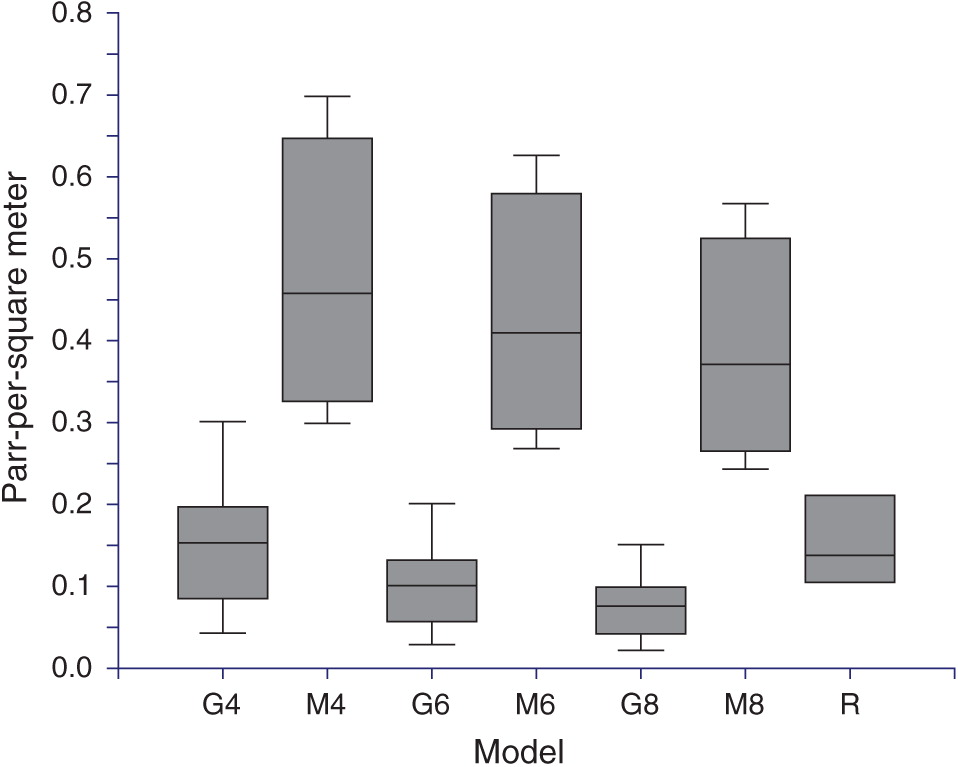
The rearing densities from Gibbons et al. (1985) rescaled to our three estimates of main channel rearing widths average 0.086 parr·m−2 (width = 8 m) to 0.173 parr·m−2 (width = 4 m). Our adjusted parr density estimates range from 0.243 parr·m−2 for the most productive high marine survival scenario and maximum rearing channel width of 8 m (model H4, Table 3) to 0.698 parr·m−2 for the least productive low marine survival scenario and minimum rearing channel width of 4 m (model L1, Table 3). The mean of the four low marine survival scenarios across the three rearing channel widths ranges from 0.492 to 0.606 parr·m−2, and for the four high marine survival scenarios ranges from 0.285 to 0.351 parr·m−2 (Table 3). The average density over all eight models ranges from 0.388 to 0.478 parr·m−2. Thus, our model-based estimates of mainstem parr rearing densities circa 1895 are 2.8–4.5 times the rescaled densities estimated by Gibbons et al. (1985) for main channel rearing habitats. It is worth noting, however, that the parr count for one of Gibbons et al.’s main channel sites (Sol Duc 2, Supplementary Material 3, Table S4) rescaled to our shallow shoreline rearing widths results in densities ranging from 0.279 to 0.557 parr·m−2, which spans the range of densities estimated by most of our eight models. So, this site at the time that it was surveyed in the early 1980s shows that densities in main channel rearing habitats are capable of achieving the densities estimated by our model. We conclude that our model-based estimates of total parr production required to produce the Stillaguamish River 1895 equilibrium are not unrealistically high.
Relevance for conservation of Puget Sound steelhead
Although there are data showing that declines in the productivity of the marine environment in recent decades have impaired the recruitment of steelhead on a regional basis (Ward and Slaney 1988; Smith et al. 2000; Ward 2000; Friedland et al. 2014; Moore et al. 2015), considerably less is known about how alterations of freshwater habitats have affected juvenile production. In general, little is known about where in the freshwater life cycle from egg deposition to smolt emigration key bottlenecks are located. Nonetheless, the majority of remedial actions directed at recovering Puget Sound steelhead are most likely to be directed at freshwater habitat conditions (NMFS 2013). Partitioning the life history between the freshwater and marine phases of the life cycle in our model facilitates the identification of conditions that can result in positive population growth (λ > 1). In particular, it should facilitate the identification of minimum spawner-to-smolt survival rates necessary to achieve positive population growth under varying marine survival scenarios. This is well-illustrated by the contrast in equilibrium fry-to-parr survival rates between our low and high marine survival scenarios (Table 1; Supplementary Material 1, Table S3), where lower marine survival requires higher fry-to-parr survival rates (weaker density dependent fry mortality, greater total fry capacity) than when marine survival rates are higher.
The results from our modeling effort suggest that measuring and monitoring the parr capacity of rearing habitats by measuring parr density provides an integrative metric of population performance within the entire freshwater life cycle. It can provide the most direct link between remedial actions aimed to improve the quantity and quality of rearing habitats and improvements in survival to a critical early juvenile life stage, age-1 parr. Consequently, quantifying parr capacities and parr-to-smolt survival rates are key information needs for recovery planning. In addition, estimates of spawner age composition and size-specific fecundity can provide estimates of potential egg deposition that when combined with estimates of parr production can provide estimates of egg-to-parr survival. Developing credible estimates of egg-to-parr and parr-to-smolt survival rates should help to focus scarce recovery resources on the most appropriate habitat actions to undertake in order to improve survival across the total life cycle, particularly given limited ability (in the near term at least) to affect improvements in marine survival.
Our model-based estimates of parr densities in 1895 provide a credible baseline from which all these issues can be addressed. To illustrate the value of achieving the higher parr densities estimated from our model, Table 5 shows the adult returns expected from achieving mean parr densities from the lower range of our model estimates given the amount of rearing habitat in the Stillaguamish River estimated to be currently available. We assumed parr-to-smolt survival of 0.3 (Hard et al. 2015), and smolt-to-adult return survival of 0.03, which is below the recent average for the Keogh estimated by Friedland et al. (2014) and likely near values achieved by wild steelhead in northern Puget Sound rivers within the past decade.
Table 5.
| Habitat type | Area (m2) | Density 1 (parr·m−2): 0.24 | Density 2 (parr·m−2): 0.32 | Density 3 (parr·m−2): 0.4 |
|---|---|---|---|---|
| Tributaries + mainstem 1 | 1 023 799 | 2211 | 2949 | 3686 |
| Tributaries + mainstem 2 | 1 259 301 | 2720 | 3627 | 4533 |
| Tributaries + mainstem 3 | 1 494 803 | 3229 | 4305 | 5381 |
Depending on the width of shallow shoreline rearing habitat, average rearing densities of 0.24 parr·m−2 in tributaries and mainstem combined could recruit 2200–3200 adults at a smolt-to-adult survival rate of 0.03. Average rearing densities of 0.4 parr·m−2 would recruit 3700–5400. Clearly, achieving such modest mean parr rearing densities would achieve significant improvements in wild steelhead recruitment in the Stillaguamish River, and elsewhere in Puget Sound, relative to current levels of abundance (Ford 2011; Hard et al. 2015).
Changes in the adult steelhead population since 1895 and the value of repeat spawning.
Our model of the 1895 steelhead population assumed a more complex age-structure than exists today in the Stillaguamish River, particularly with respect to the degree of repeat spawning. The model also assumed four mature ages, 3–6, with the proportions at equilibrium dominated by the two older age classes, which combined accounted for 70% of annual returns at equilibrium. These assumptions resulted in an average fecundity (eggs/female) of the modeled populations of 4800 and 4900 for the two marine survival scenarios (Table 1; Supplementary Material 1, Table S3), which are essentially identical to the average value for steelhead generally noted by Quinn (2005). The contemporary population has a much lower, perhaps negligible, percentage of repeat spawners (Hard et al. 2015), and is dominated by age-3- and age-4-year-old individuals (Hard et al. 2007). This undoubtedly has reduced the average fecundity of the population and thus the total potential egg deposition.
These changes in the age- and life-history structure of the contemporary population, however, do not affect the validity of our results as the purpose of the modeling is to provide estimates of the abundance of parr and the associated rearing densities that were most likely responsible for the level of adult equilibrium abundance in 1895 estimated by Gayeski et al. (2011). These estimates are directly relevant to conservation planning for Stillaguamish and other Puget Sound steelhead populations. As illustrated in the preceding subsection and Table 5, attaining higher rearing densities in the Stillaguamish River is directly relevant to the recovery of the steelhead population. So also is recovering the historic proportion of repeat spawners. Repeat spawning is likely to be especially important for recovery of Puget Sound steelhead given current depressed levels of marine survival, which primarily affects steelhead smolts early during the first year in the marine environment (Friedland et al. 2014; Moore et al. 2015). Post-spawning adults are likely to be much less susceptible to marine mortality upon re-entering the marine environment than much smaller bodied smolts and their return to spawn a second time achieves a functional increase in the effective cohort smolt-to-adult survival rate, as shown in Table 1 and Supplementary Material 1, Table S3. A significant increase in the proportion of repeat spawners to levels in the neighborhood of 20% of total annual spawners could be critical to achieving the increase in parr densities that our modeling results show to be realistic. It is worth noting in this regard that according to recent run reconstruction data provided to the lead author by Washington Department of Fish and Wildlife staff, repeat spawning rates of winter-run steelhead in the Queets River in Olympic National Park to the west of Puget Sound have ranged between 20% and 30% since the early 1980s. So such repeat spawning rates are still achievable today at least by some populations.
Regardless of the recovery of greater rates of repeat spawning, increasing the mean densities of steelhead parr in the Stillaguamish River can be expected to return significant dividends for rebuilding depressed levels of adult abundance of this population. Even modest increases to densities above 0.2 parr·m−2 should yield meaningful sustained increases in the abundance of returning adults. Achieving such increases will require both improvements to habitat quality and quantity (physical structure and complexity, and food web) and synergistic increases in the numbers of returning adult spawners. The results of our modeling of the parr capacity of the Stillaguamish River in 1895 show that such historic levels of parr density were not extreme by comparison with many studied populations today and that it is not unreasonable to expect to attain such densities in rivers today if appropriate recovery actions are undertaken.
Conclusion
Our life-cycle model estimates of the abundance of steelhead parr that was likely required to achieve the 1895 adult return of steelhead to the Stillaguamish River relied on conservative assumptions regarding spawning and pre-smolt survival in freshwater and a conservative range of post-smolt marine survival. These assumptions obviously lead to higher estimates of steelhead parr capacity and rearing densities in the Stillaguamish than if we had assumed either a smaller number of returning adults or greater post-smolt marine survival rates. However, our model estimates of total parr production equate to average parr rearing densities of 0.24–0.70 parr·m−2, which is within the range of densities that have recently been reported for relatively un-impacted streams and rivers in the Pacific northwest (0.16–0.9 m−2) (Harvey et al. 2005; McCarthy et al. 2009; Harston and Kennedy 2015).
Steelhead parr densities in the few Puget Sound rivers that have been studied are currently well below even the lowest densities estimated by our model, consistent with currently reduced levels of adult abundance. Our results strongly indicate that attaining even the lowest densities estimated by our model can achieve a significant increase in parr numbers and, hence, numbers of smolts and returning adults. Increasing smolt abundance is particularly important in view of current rates of smolt-to-adult returns that are well-below averages rates in the 1980s.
Acknowledgements
Dr. Corey Phillis and Dr. Richard Zabel provided helpful comments on a preliminary draft of the manuscript. We are grateful to two anonymous reviewers and the editor for comments that greatly improved the submitted manuscript. We also extend our thanks to Oleksandr Stevankiv, an NOAA contractor who works with the National Marine Fisheries Service at the Northwest Fisheries Science Center for creating the map in Fig. 1 specifically for this publication. No special funding was required for this project. The lead author undertook the majority of the work for this publication, including all of the modeling, preparation of the text, and the majority of the editing on his personal time. The contributions of co-authors Pess and Beechie were provided as part of their regular work load at NMFS’ Northwest Fisheries Science Center, Fish Ecology Division.
References
Beechie TJ, Pess G, Beamer E, Lucchetti G, and Bilby RE. 2003. Role of watershed assessments in recovery planning for endangered salmon. In Restoration of Puget Sound Rivers. Edited by D Montgomery, S Bolton, D Booth, and L Wall. University of Washington Press, Seattle, WA. pp. 194–225.
Beechie T, Pess G, Morley S, Butler L, Downs P, Maltby A, Skidmore P, Clayton S, Muhlfeld C, and Hanson K. 2013. Chapter 3: watershed assessments and identification of restoration needs. In Stream and watershed restoration: a guide to restoring riverine processes and habitats. Edited byP Roni, and T Beechie. Wiley-Blackwell, Chichester, UK. pp. 50–113.
Beechie TJ, Sear D, Olden J, Pess GR, Buffington J, Moir H, Roni P, and Pollock MM. 2010. Process-based principles for restoring river ecosystems. BioScience, 60: 209–222.
Brault S, and Caswell H. 1993. Pod-specific demography of killer whales (Orcinus orca). Ecology, 74(5): 1444–1454.
Ford MJ (ed.). 2011. Status review update for Pacific salmon and steelhead listed under the Endangered Species Act: Pacific Northwest. NOAA Technical Memorandum NMFS-NWFSC-113, U.S. Department of Commerce. 281 p.
Friedland KD, Ward BR, Welch DW, and Hayes SA. 2014. Postsmolt growth and thermal regime define the marine survival of steelhead from the Keogh River, British Columbia. Marine and Coastal Fisheries: Dynamics, Management, and Ecosystem Science, 6: 1–11.
Gayeski N, McMillan B, and Trotter P. 2011. Historical abundance of Puget Sound steelhead, Oncorhynchus mykiss, estimated from catch record data. Canadian Journal of Fisheries and Aquatic Sciences, 68(3): 498–510.
Gibbons RG, Hahn PKJ, and Johnson TH. 1985. Methodology for determining MSH steelhead spawning escapement requirements. Fisheries Management Division Report 85-11, Washington State Game Department, Olympia, WA. 39 p.
Greene C, and Beechie TJ. 2004. Consequences of potential density-dependent mechanisms on recovery of ocean-type chinook salmon (Oncorhynchus tshawytscha). Canadian Journal of Fisheries and Aquatic Sciences, 61: 590–602.
Hard JJ, Myers JM, Connor EJ, Hayman RA, Kope RG, Lucchetti G, Marshall AR, Pess GR, and Thompson BE. 2015. Viability criteria for steelhead within the Puget Sound distinct population segment. NOAA Technical Memorandum NMFS-NWFSC-129. U.S. Department of Commerce.
Hard JJ, Myers JM, Ford MJ, Cope RG, Pess GR, Waples RS, Winans GA, Berejikian BA, Waknitz FW, Adams PB, Bisson PA, Campton DE, and Reisenbichler RR. 2007. Status review of Puget Sound steelhead (Oncorhynchus mykiss). NOAA Technical Memorandum NMFS-NWFSC-81. U.S. Department of Commerce. 117 p.
Harston RB, and Kennedy BP. 2015. Competitive release modifies the impacts of hydrological alteration for a partially migratory stream predator. Ecology of Freshwater Fish, 24(2): 276–292.
Harvey BC, White JL, and Nakamoto RJ. 2005. Habitat-specific biomass, survival, and growth of rainbow trout (Oncorhynchus mykiss) during summer in a small coastal stream. Canadian Journal of Fisheries and Aquatic Science, 62(3): 650–658.
McCarthy SG, Duda JJ, Emlen JM, Hodgson GR, and Beauchamp DA. 2009. Linking habitat quality and trophic performance of steelhead along forest gradients in the South Fork Trinity River watershed, California. Transactions of the American Fisheries Society, 138: 506–521.
McElhany P, Ruckelshaus MH, Ford MJ, Wainwright TC, and Bjorkstedt EP. 2000. Viable salmonid populations and the recovery of evolutionarily significant units. NOAA Technical Memorandum NMFS-NWFSC-42. U.S. Department of Commerce. 156 p.
McGurk MD. 1996. Allometry of marine mortality of Pacific salmon. Fishery Bulletin, 94: 77–88.
Moore ME, Berejikian BA, Goetz FA, Berger AG, Hodgson SS, Connor EJ, and Quinn TP. 2015. Multi-population analysis of Puget Sound steelhead survival and migration behavior. Marine Ecology Progress Series, 537: 217–232.
Myers JM, Hard JJ, Connor EJ, Hayman RA, Kope RG, Lucchetti G, Marshall AR, Pess GR, and Thompson BE. 2015. Identifying historical populations of steelhead within the Puget Sound distinct population segment. NOAA Technical Memorandum NMFS-NWFSC-128. U.S. Department of Commerce.
NMFS. 2010. National marine fisheries service interim endangered and threatened species recovery planning guidance version 1.3. National Marine Fisheries Service, Silver Spring, MD. Available from www.nmfs.noaa.gov/pr/pdfs/recovery/guidance.pdf.
NMFS. 2013. Federal recovery outline, Puget Sound distinct population segment. National Marine Fisheries Service, Northwest Regional Office, Seattle, WA.
Olesiuk PF, Ellis GM, and Ford JKB. 2005. Life history and population dynamics of northern resident killer whales (Orcinus orca) in British Columbia. Canadian Science Advisory Secretariat 2005/045. Fisheries and Oceans Canada.
Oosterhout GR, Huntington CW, Nickelson TE, and Lawson PW. 2005. Potential benefits of a conservation hatchery program for supplementing Oregon coast coho salmon (Oncorhynchus kisutch) populations: a stochastic model investigation. Canadian Journal of Fisheries and Aquatic Sciences, 62: 1920–1935.
Pavlov DS, Savvaitova KA, Kuzischin KV, Gruzdeva MA, Pavlov SD, Mednikov BM, and Maksimov SV. 2001. The Pacific noble salmons and trouts of Asia. Scientific World, Moscow.
Pess G, Collins B, Pollock MM, Beechie TJ, Haas AD, and Grigsby S. 1999. Historic and current factors that limit coho salmon (Oncorhynchus kisutch) production in the Stillaguamish River basin Washington State: implications for salmonid habitat protection and restoration. Report to the Snohomish County Department of Public Works, Surface Water Management Division, The Stillaguamish Tribe, Everett, WA.
Pess GR, Kiffney PM, Liermann MC, Bennett TR, Anderson JH, and Quinn TP. 2011. The influences of body size, habitat quality, and competition on the movement and survival of juvenile coho salmon during the early stages of stream recolonization. Transactions of the American Fisheries Society, 140: 883–897.
Pollock MM, Pess GR, Beechie TJ, and Montgomery DR. 2004. The importance of beaver ponds to coho salmon production in the Stillaguamish River Basin, Washington, USA. North American Journal of Fisheries Management, 24: 749–760.
Quinn T. 2005. The behavior and ecology of Pacific salmon and trout. American Fisheries Society, Bethesda, Maryland, in association with University of Washington Press, Seattle and London.
Roni P, Pess G, Beechie T, and Morley S. 2010. Estimating changes in coho salmon and steelhead abundance from watershed restoration: how much restoration is needed to measurably increase smolt production? North American Journal of Fisheries Management, 30: 1469–1484.
Scheuerell MD, Hilborn R, Ruckelshaus MH, Bartz KK, Lagueux KM, Haas AD, and Rawson K. 2006. The Shiraz model: a tool for incorporating anthropogenic effects and fish–habitat relationships in conservation planning. Canadian Journal of Fisheries and Aquatic Sciences, 63: 1596–1607.
Seamons TR, Bentzen P, and Quinn TP. 2004. The mating system of steelhead, Oncorhynchus mykiss, inferred by molecular analysis of parents and progeny. Environmental Biology of Fishes, 69: 333–344.
Smith BD, Ward BR, and Welch DW. 2000. Trends in wild adult steelhead (Oncorhynchus mykiss) abundance in British Columbia as indexed by angler success. Canadian Journal of Fisheries and Aquatic Sciences, 57: 255–270.
Stanford JA, Lorang MS, and Hauer FR. 2005. The shifting habitat mosaic of river ecosystems. Verhandlungen des Internationalen Verein Limnologie, 29: 1–14.
Tear TH, Kareiva P, Angermeier PL, Comer P, Czech B, Kautz R, Landon L, Mehlman D, Murphy K, Ruckelshaus M, Scott JM, and Wilhere G. 2005. How much is enough? The recurrent problem of setting measurable objectives in conservation. BioScience, 55(10): 835–849.
Ward BR. 2000. Declivity in steelhead (Oncorhynchus mykiss) recruitment at the Keogh River over the past decade. Canadian Journal of Fisheries and Aquatic Sciences, 57: 298–306.
Ward BR, and Slaney PA. 1988. Life history and smolt-to-adult survival of Keogh River steelhead trout (Salmo gairdneri) and the relationship to smolt size. Canadian Journal of Fisheries and Aquatic Sciences, 45: 1110–1122.
Ward BR, and Slaney PA. 1993. Egg-to-smolt survival and fry-to-smolt density dependence of Keogh River steelhead trout. In Production of juvenile Atlantic salmon, Salmo salar, in natural waters. Edited by RJ Gibson, and RE Cutting. Canadian Special Publication of Fisheries and Aquatic Sciences no. 118, pp. 209–217.
Welch DW, Ward BR, Smith BD, and Everson JP. 2000. Temporal and spatial responses of British Columbia steelhead (Oncorhynchus mykiss) populations to ocean climate shifts. Fisheries Oceanography, 9: 17–32.
Wilcox WA. 1898. Notes on the fisheries of the Pacific coast in 1895. In Report of the commissioner for the year ending June 30, 1896, Part XXII. US Commission of Fish and Fisheries, Washington, D.C. pp. 575–613.
Withler IL. 1966. Variability in life history characteristics of steelhead trout (Salmo gairdneri) along the Pacific coast of North America. Journal of the Fisheries Research Board of Canada, 23(3): 365–393.
Supplementary material
Supplementary Material 1(PDF / 56.4 KB):
- Download
- 56.42 KB
Supplementary Material 2(PDF / 6.48 KB):
- Download
- 6.49 KB
Supplementary Material 3(PDF / 12.4 KB):
- Download
- 12.43 KB
Information & Authors
Information
Published In

FACETS
Volume 1 • Number 1 • January 2017
Pages: 83 - 104
Editor: Steven Cooke
History
Received: 11 December 2015
Accepted: 16 April 2016
Version of record online: 14 July 2016
Copyright
© 2016 Gayeski et al. This work is licensed under a Creative Commons Attribution 4.0 International License (CC BY 4.0), which permits unrestricted use, distribution, and reproduction in any medium, provided the original author(s) and source are credited.
Data Availability Statement
All relevant data are within the paper and in the Supplementary Material.
Key Words
Sections
Subjects
Authors
Author Contributions
All conceived and designed the study.
All performed the experiments/collected the data.
NG analyzed and interpreted the data.
All contributed resources.
NG drafted or revised the manuscript.
Competing Interests
The authors have declared that no competing interests exist.
Metrics & Citations
Metrics
Other Metrics
Citations
Cite As
Nick Gayeski, George Pess, and Tim Beechie. 2017. A life-table model estimation of the parr capacity of a late 19th century Puget Sound steelhead population. FACETS.
1(): 83-104. https://doi.org/10.1139/facets-2015-0010
Export Citations
If you have the appropriate software installed, you can download article citation data to the citation manager of your choice. Simply select your manager software from the list below and click Download.
There are no citations for this item