Measuring statistical evidence and multiple testing
Abstract
The measurement of statistical evidence is of considerable current interest in fields where statistical criteria are used to determine knowledge. The most commonly used approach to measuring such evidence is through the use of p-values, even though these are known to possess a number of properties that lead to doubts concerning their validity as measures of evidence. It is less well known that there are alternatives with the desired properties of a measure of statistical evidence. The measure of evidence given by the relative belief ratio is employed in this paper. A relative belief multiple testing algorithm was developed to control for false positives and false negatives through bounds on the evidence determined by measures of bias. The relative belief multiple testing algorithm was shown to be consistent and to possess an optimal property when considering the testing of a hypothesis randomly chosen from the collection of considered hypotheses. The relative belief multiple testing algorithm was applied to the problem of inducing sparsity. Priors were chosen via elicitation, and sparsity was induced only when justified by the evidence and there was no dependence on any particular form of a prior for this purpose.
Introduction
The need for the measurement of statistical evidence arises as an issue in science as follows. The scientific problem under consideration concerns some quantity of interest for which an investigator either wants to know its value or has a hypothesis that the quantity takes a specific value and wants to know if this is true or false. To answer such a question data x are collected. It is rare that the data provide a definitive answer but it is believed that the data contain evidence concerning this. The purpose of statistical reasoning or inference is to use this evidence to estimate the quantity of interest and provide an assessment of the accuracy of the estimate or indicate whether there is evidence either in favor of or against the hypothesized value, and provide an assessment of the strength of this evidence.
To implement statistical inference, additional ingredients are required. First, it is presumed that the data x can be thought of as having arisen from a probability distribution as represented by the density f. Provided the data were collected properly, this assumption is reasonable and this is assumed here. A consequence of this is that the data can be thought of as being objective in the sense that f fully describes how the data were produced from the set of possible data values. Of course, f is generally not known so it is assumed that f ∈ {fθ : θ ∈ Θ}, a family of probability densities on referred to as the statistical model. Here θ is called the parameter and Θ the parameter space of the model. The quantity of interest is then represented as ψ = Ψ(θ), where Ψ:Θ → Ψ, and we don’t distinguish between the function and its range to save notation.
A natural approach to constructing a theory of inference is to determine a measure of the evidence in the data x that ψ is the true value for each ψ ∈ Ψ. The value ψ(x) ∈ Ψ that maximizes this measure of evidence is, then, the obvious estimate and a subset C(x) ⊂ Ψ of values with evidence measures above some threshold would, through a measure of its size, serve to give an assessment of the accuracy of ψ(x). For a null hypothesis H0 : Ψ(θ) = ψ0 the measure of evidence at ψ0 indicates whether there is evidence in favor of or against H0 and a measure of the strength of this evidence is then obtained by comparing the evidence at ψ0 with the evidence at each of the other possible values for ψ. A theory that accomplishes this, based on the relative belief ratio RB(ψ | x) as the measure of evidence, is described by Evans (2015) and outlined in the section “Statistical analysis based on relative belief”.
Even though p-values are commonly used to measure evidence, it has long been recognized that there are serious issues associated with their use (for example, see Royall (1997)). This can be readily observed by considering what the cutoff is to determine when there is evidence against or for a hypothesis. Cutoffs like 5% are not only arbitrary, many treatments of p-values insist that it is not possible for a p-value to give evidence in favor of a null hypothesis. Although that is a perfectly valid statement, it seems like a significant weak point for a supposed measure of evidence. Even when a very small p-value is observed this does not mean that a result of scientific interest has been obtained. For, given the finite accuracy with which measurements are taken, it is rarely the case that the truth of H0 practically corresponds to an exact value ψ0. Rather, there is a region about ψ0 such that if the true value lies in this region, for all practical purposes, H0 is true. Using relative belief ratios evidence can be obtained either for or against H0, there is a clear measure of the strength of the evidence, and the essential discreteness involved in assessing H0 is easily handled.
The theory of relative belief requires an additional ingredient, namely a prior probability distribution π must be specified on Θ that reflects the beliefs concerning what values of θ are more or less likely. The prior is determined by an elicitation algorithm that is an argument as to why the prior in question is to be considered suitable. The prior π is subjective in nature and that seems contrary to the dictates of science, which properly has objectivity as the goal. Although it doesn’t justify the use of priors, it is to be noted that the model {fθ : θ ∈ Θ} is also subjective as it is chosen by the investigator. One could argue in favor of this subjectivity, however, particularly when the choices are being made by an expert, as informed input should result in a better analysis, but doubts linger. Part of our approach to dealing with this concern is to check that any ingredient chosen is not contradicted by the objective data. Therefore, model checking and checking for prior–data conflict are necessary. Also, it is possible to choose a prior such that a desired result is obtained but such bias can be measured and controlled a priori by design. Some discussion on assessing prior–data conflict and bias is provided in the section “Statistical analysis based on relative belief”.
The focus of this paper is the following problem. Suppose Ψ is an open subset of Rk and we wish to assess the individual hypotheses H0i = {θ : Ψi(θ) = ψ0i}, namely H0i is the hypothesis that the i-th coordinate of ψ equals ψ0i. Considering these hypotheses separately is the multiple testing problem and the concern is to ensure that while controlling the individual error rate, the overall error rate is not too large. An error means either the acceptance of H0i when it is false (a false negative) or the rejection of H0i when it is true (a false positive). One approach is to make an inference about the number of H0i that are true (or false) and then use this to control the number of H0i that are accepted (or rejected). In the section “Inferences for multiple tests”, this is shown to work for small k but to fail for large k. As a remedy for this, a relative belief multiple testing algorithm is developed that controls for false positives and false negatives through the use of bounds on the evidence that are determined by the measurement of bias. This approach is shown to be consistent and to possess an optimal property when considering the assessment of a randomly selected hypothesis from the set of hypotheses.
In the section “Applications”, an application is made of the relative belief multiple testing algorithm to the problem of inducing sparsity. If it is known that ψi = Ψi(θ) = ψ0i, then the effective dimension of the quantity of interest is k − 1, which is a simplification of the model. Sometimes there is a belief that many of the hypotheses H0i are true, but there is little prior knowledge about which are true and it is, therefore, not clear how to choose a prior that reflects this belief. A common approach is to use a prior that, together with a particular estimation procedure, forces many of the ψi to take the corresponding value ψ0i. For example, the use of a Laplace prior together with using the maximum value of the posterior as the estimate, known as maximum a posteriori (MAP) estimation, is known to accomplish this for certain problems. Problems with this approach include the possibility that such an assignment is simply an artifact of the prior and the estimation procedure and that sparsity requires an overly concentrated prior that leads to prior–data conflict with the coordinates for which H0i is rejected. It would be preferable to have a procedure that was not dependent on a specific form for the prior, avoided prior–data conflict, and was based on the statistical evidence contained in the data, and this is the approach taken here. Practical applications are presented, with special emphasis on regression problems including the situation where the number of predictors exceeds the number of observations.
Evans (2015) noted that there are connections between relative belief and the pure likelihood approach to inference, as both consider statistical evidence as the core concept. This is also reflected in the approach to multiple testing developed in the current paper and that discussed by Strug and Hodge (2006a, 2006b). There have been several priors proposed for the sparsity problem through MAP estimation; for example, the spike-and-slab prior discussed by George and McCulloch (1993) and Rockova and George (2014), the Laplace prior discussed by Park and Casella (2008), and the horseshoe prior of Carvalho et al. (2009). Any prior can be used with the approach taken here, but logically an elicited prior is preferred over one possessing certain properties.
Statistical analysis based on relative belief
Suppose that interest is in inference about the quantity Ψ(θ) = ψ. Let ΠΨ denote the prior measure of ψ, with density πΨ, and let ΠΨ(⋅ | x) denote the posterior measure of ψ, with density πΨ(⋅ | x). Evidence is measured by change in belief (for example, see Salmon (1973) or Howson and Urbach (2006)), thus if belief in ψ increases there is evidence in favor of this value and evidence against it if belief decreases. Evans (2015) argued for the relative belief ratio RBΨ(ψ | x) = limδ→0ΠΨ(Nδ(ψ) | x)/ΠΨ(Nδ(ψ)) as a measure of evidence, where Nδ(ψ) is a sequence of neighborhoods of ψ converging (nicely, as defined by Rudin (1974)) to {ψ} as δ → 0. When πΨ and πΨ(⋅ | x) are continuous at ψ, thenSo RBΨ(ψ | x) > 1 indicates evidence in favor of ψ, RBΨ(ψ | x) < 1 indicates evidence against, and RBΨ(ψ | x) = 1 gives no evidence either way. Any 1−1 increasing function of RBΨ(⋅ | x) is an equivalent measure of evidence and RBΨ(⋅ | x) is invariant under smooth reparameterizations, thus relative belief inferences are invariant to these choices.
(1)
The best estimate of ψ is the value that maximizes the evidence, namely ψ(x) = arg sup RBΨ(ψ | x). Associated with this is a γ-credible region CΨ, γ(x) = {ψ : RBΨ(ψ | x) ≥ cΨ, γ(x)} containing those values whose evidence is above the threshold cΨ, γ(x) = inf{k : ΠΨ(RBΨ(ψ | x) > k | x) ≤ γ}. As ψ(x) ∈ CΨ, γ(x), for every γ ∈ [0, 1], for selected γ, the “size” of CΨ, γ(x) is a measure of the accuracy of ψ(x). A calibration of RBΨ(ψ0 | x) is given by the strengthWhen RBΨ(ψ0 | x) < 1, a small value of eq. (2) indicates a large posterior belief that the true value has a relative belief ratio greater than RBΨ(ψ0 | x), and therefore there is strong evidence against ψ0 but only weak evidence against it if eq. (2) is big. If RBΨ(ψ0 | x) > 1, a large value of eq. (2) indicates a small posterior probability that the true value has a relative belief ratio greater than RBΨ(ψ0 | x), and therefore there is strong evidence in favor of ψ0, whereas a small value of eq. (2) only indicates weak evidence in favor of ψ0. A variety of optimality and consistency results have been established for these inferences (see Evans (2015)).
(2)
When H0 : Ψ(θ) = ψ0 is false both eqs. (1) and (2) converge to 0, and when H0 is true then eq. (1) converges to the maximum possible value, which is always >1. When H0 is true and there are only a finite number of possible values for ψ then eq. (2) converges to 1, but in the continuous case eq. (2) can converge to a U(0,1) distribution. The view is taken here, however, that any time continuous probability is used this is an approximation to a finite, discrete context. For example, if ψ is a mean and the response measurements are to the nearest centimeter, then of course the true value of ψ cannot be known to an accuracy >0.5 cm, no matter how large the sample is. Furthermore, there are implicit bounds associated with any measurement process. As such, the restriction can be made to discretized parameters that take only a finite number of values. Thus, when ψ is a continuous, real-valued parameter, it is discretized to the intervals …, (ψ0 − 3δ/2, ψ0 − δ/2], (ψ0 − δ/2, ψ0 + δ/2], (ψ0 + δ/2, ψ0 + 3δ/2], … for some choice of δ > 0, and there are only a finite number of such intervals covering the range of possible values. With this discretization, then H0 = (ψ0 − δ/2, ψ0 + δ/2] and eq. (2) is consistent. Thus, δ needs to be specified as part of the application, at least when the goal is assessing the evidence concerning H0. The value of δ is simply the smallest difference from ψ0 that matters in the application and presumably a knowledgeable scientist knows what this is and designs the measurement process that produces the data accordingly.
Let be such that H0 is accepted whenever x ∈ A, thus, with M(⋅ | H0) denoting the prior predictive measure given that H0 is true, M(A | H0) is the prior probability of accepting H0 when it is true. The relative belief acceptance region is Arb(ψ0) = {x : RBΨ(ψ0 | x) > 1}. Let be such that H0 is rejected whenever x ∈ R and the relative belief rejection region is Rrb(ψ0) = {x : RBΨ(ψ0 | x) < 1}. Letting M denote the unconditional prior predictive measure the following result was proved by Evans (2015).
Theorem 1: (i) The acceptance region Arb(ψ0) minimizes M(A) among all acceptance regions A, satisfying M(A | H0) ≥ M(Arb(ψ0) | H0). (ii) The rejection region Rrb(ψ0) maximizes M(R) among all rejection regions R, satisfying M(R | H0) ≤ M(Rrb(ψ0) | H0).
The implication of this is that, when ΠΨ({ψ0}) = 0, then Arb(ψ0) minimizes the prior probability that H0 is accepted given that it is false among all acceptance regions A satisfying the condition in (i) and Rrb(ψ0) maximizes the prior probability that H0 is rejected given that it is false among all rejection regions R satisfying the condition in (ii). The same result holds for the case when ΠΨ({ψ0}) > 0 with the inequalities in (i) and (ii) replaced by equalities. Under independent identically distributed (IID) sampling, M(Arb(ψ0) | H0) → 1 and M(Rrb(ψ0) | H0) → 0 as sample size increases, so these quantities can be controlled by design. Theorem 1 can be generalized to obtain optimality results for the acceptance region Arb, q(ψ0) = {x : RBΨ(ψ0 | x) > q} and the rejection region Rrb, q(ψ0) = {x : RBΨ(ψ0 | x) < q}. The following inequality is useful in the section “Inferences for multiple tests” in controlling error rates.
Theorem 2: M(Rrb, q(ψ0) | ψ0) ≤ q.
Proof: By the Savage–Dickey result (see proposition 4.2.7 in Evans (2015)), RBΨ(ψ0 | x) = m(x | ψ0)/m(x). Now , and therefore, by Markov’s inequality, M(Rrb,q(ψ0) | ψ0) = M(m(x)/m(x | ψ0) > 1/q | ψ0) ≤ q.
One of the key concerns with Bayesian inference methods is that the prior can bias the analysis. Given a measure of evidence, however, it is possible to measure and control bias. The bias against H0 is given by M(RBΨ(ψ0 | x) ≤ 1 | ψ0) = 1−M(Arb(ψ0) | ψ0) as this is the prior probability that evidence will be obtained against H0 when it is true. If the bias against H0 is large, subsequently reporting, after seeing the data, that there is evidence against H0 is not convincing. The bias in favor of H0 is given by for values such that the difference between ψ0 and represents the smallest difference of practical importance; note that this tends to decrease as moves farther away from ψ0. When the bias in favor is large, subsequently reporting, after seeing the data, that there is evidence in favor of H0 is not convincing. For a fixed prior, both biases decrease with sample size and thus, in design situations, they can be used to set sample size and thereby control bias.
It is never known that the ingredients chosen for a statistical analysis are correct, but hopefully these serve as useful approximations in the sense that inferences drawn from them are reasonably accurate. If x lies in the tails of fθ for every θ ∈ Θ, then it can be concluded that there is a problem with the model and it needs to be modified. It is clear that checking the prior is a meaningless activity if the model is to be discarded, thus model checking is carried out first. If the model passes, then the prior is checked and the approach of Evans and Moshonov (2006) is adopted here. For this let T be a minimal sufficient statistic (MSS) for the model with density mT, and if the probability MT(mT(t) ≤ mT(T(x))) is small, then conclude a prior–data conflict exists as this says that T(x) lies in the tails of the prior-predictive. The consistency of this procedure was established by Evans and Jang (2011a) as, under weak conditions this probability converges to Π(π(θ) ≤ π(θtrue)), and a methodology for modifying a prior that fails its checks was developed by Evans and Jang (2011b).
Inferences for multiple tests
Consider now the multiple testing problem. The typical approach to this problem relies on the use of p-values that, for the reasons discussed, are not adopted here. Rather, the relative belief ratio as a valid measure of statistical evidence is used as the basis for all inferences.
To see what the problem is with multiple testing suppose that Ψi is finite for each i, perhaps arising via a discretization as discussed in the section “Statistical analysis based on relative belief”, and let be the proportion of the hypotheses H0i that are true. Note that the discreteness is essential, otherwise, under a continuous prior on Ψ, the prior distribution of Ξ(θ) is degenerate at 0. In an application it is desirable to make inference about the true value of ξ ∈ Ξ = {0, 1/k, 2/k,…, 1} and this is based on the relative belief ratio RBΞ(ξ | x) = Π(Ξ(θ) = ξ | x)/Π(Ξ(θ) = ξ). The appropriate estimate of Ξ is ξ(x) = arg supξRBΞ(ξ | x) and its accuracy is assessed using the size of CΞ, γ(x) for some choice of γ ∈ [0, 1]. Hypotheses such as H0 = {θ : Ξ(θ) ∈ [ξ0, ξ1]}, namely the proportion true is at least ξ0 and no greater than ξ1, is assessed using the relative belief ratio RB(H0 | x) = Π(ξ0 ≤ Ξ(θ) ≤ ξ1 | x)/Π(ξ0 ≤ Ξ(θ) ≤ ξ1), which equals RBΞ(ξ0 | x) when ξ0 = ξ1.
The estimate ξ(x) can be used to control how many hypotheses are potentially accepted. For this, select kξ(x) of the H0i as being true from among those for which RBΨi(ψ0i | x) > 1. Note that it does not make sense to accept H0i when RBΨi(ψ0i | x) < 1 as there is evidence against H0i. Thus, if there are fewer than kξ(x) satisfying RBΨi(ψ0i | x) > 1, then fewer than this number should be accepted. If there are more than kξ(x) of the relative belief ratios satisfying RBΨi(ψ0i | x) > 1, then some method will have to be used to select the kξ(x) that are potentially accepted. It is clear, however, that the logical way to do this is to order the H0i, for which RBΨi(ψ0i | x) > 1, based on their strengths ΠΨ(RBΨi(ψ0i | x) ≤ RBΨi(ψ0i | x) | x), from largest to smallest, and accept at most the kξ(x) for which the evidence is strongest. If control is desired of the number of false positives then the relevant parameter of interest is υ = ϒ(θ) = 1 − Ξ(θ), the proportion of false hypotheses. Note that Π(ϒ(θ) = υ) = Π(Ξ(θ) = 1 − υ), and therefore the relative belief estimate of υ satisfies υ(x) = 1 − ξ(x). Following the same procedure, the H0i with RBΨi(ψ0i | x) < 1 are ranked via their strengths and at most kυ(x) are rejected. This procedure will be referred to as the multiple testing algorithm.
The consistency of the multiple testing algorithm follows from results proved by Evans (2015) (see section 4.7.1 therein) under IID sampling. In other words, as the amount of data increases, ξ(x) converges to the proportion of H0i that are true, each RB(ψ0i | x) converges to the largest possible value (always >1) when H0i is true and converges to 0 when H0i is false, and the evidence in favor or against converges to the strongest possible, depending on whether the hypothesis in question is true or false.
The following example demonstrates the characteristics of the algorithm.
Example 1. Location normal.
Suppose that there are k independent samples xij for 1 ≤ i ≤ k, 1 ≤ j ≤ n, where the i-th sample is from a N(μi, σ2) distribution with μi unknown and σ2 known. It is desired to assess the evidence as to whether or not H0i : μi = μ0 is true for i = 1,…, k. It is easy to modify our development to allow the sample sizes to vary, and the case where σ2 is unknown is considered in the section “Applications”. This context is relevant to the analysis of microarray data. The statistic is an MSS for this model, and thus a natural model checking procedure is to compare the observed value of the statistic to the chi-squared(k(n − 1)) distribution.
For the prior, the μ1,…, μk are taken to be IID from a distribution. The value of is determined via elicitation. For this it is supposed that it is known with virtual certainty that each μi ∈ (ml, mu) for specified values ml ≤ mu. Here, virtual certainty is interpreted to mean that the prior probability of this interval is at least γ, where γ is a large probability like 0.99. It is also supposed that μ0 = (ml + mu)/2. This implies that λ0 = (mu − ml)/(2σΦ−1((1 + 0.99)/2)). Following Evans and Jang (2011b), increasing the value of λ0 implies a more weakly informative prior in this context and, as such, decreases the possibility of prior–data conflict, and this indicates how the prior is to be modified in case of prior–data conflict. Note that this elicitation argument also specifies μ0 when this is not predetermined. The prior distribution of T is , where 1k is the k-dimensional vector of 1s and Ik is the k × k identity matrix, and therefore the check on the prior becomes the probability , where chi-squared(k).
The posteriors of the μi are independent , where . Given that the measurements are taken to finite accuracy it is not realistic to test μi = μ0. A value δ > 0 is specified so that H0i = (μ0 − δ/2, μ0 + δ/2] in a discretization of R1 into a finite number of intervals, each of length δ, as well as two tail intervals. For some there are 2D + 1 intervals Id = (μ0 + (d − 1/2)δ, μ0 + (d + 1/2)δ] for d ∈ { −D, −D + 1,…, D} that span (ml, mu), together with the tail intervals (−∞, μ0 − (D + 1/2)δ] and (μ0 + (D + 1/2)δ, ∞). Then , with a similar formula for the tail intervals. When δ is small this is approximated by the ratio of the posterior to prior densities of μi evaluated at μ0 + dδ. Then RB(I0 | x) = RBi(H0i | x) gives the evidence for or against H0i and the strength of this evidence is computed using the discretized posterior distribution. Notice that RBi(H0i | x) converges to ∞ as λ0 → ∞ and this is characteristic of other measures of evidence such as Bayes factors. As discussed by Evans (2015), this is one of the reasons why calibrating eq. (1) via eq. (2) is necessary.
Now, consider the bias in the prior. To simplify matters, the continuous approximation is used as this makes little difference here (see Tables 3 and 4). The bias against μi = μ0 equalswhereNote that eq. (3) converges to 2(1 − Φ(1)) = 0.32 as λ0 → 0 and to 0 as λ0 → ∞ and, for fixed λ0, converges to 0 as n → ∞. Thus, there is never strong bias against μi = μ0; this is as expected because the prior is centered on μ0. The bias in favor of μi = μ0 is measured byAs λ0 → ∞ eq. (4) converges to 1, thus there is bias in favor of μi = μ0 and this reflects what was obtained for the limiting value of RBi(H0i | x). Also, eq. (4) decreases with increasing δ and goes to 0 as n → ∞; thus, bias of both types can be controlled by sample size. Perhaps the most important take away from this discussion, however, is that by using a supposedly noninformative prior with λ0 large, bias in favor of the H0i is being induced.
(3)
(4)
Consider, first, a simulated data set x when k = 10, n = 5, σ = 1, δ = 1, μ0 = 0, (ml, mu) = (−5, 5), so that λ0 = 10/2Φ−1(0.995) = 1.94 and suppose μ1 = μ2 = … = μ7 = 0, with the remaining μi = 2. The relative belief ratio function RBΞ(⋅ | x) is plotted in Fig. 1. In this case, the relative belief estimate ξ(x) = 0.70 is exactly correct. Table 1 gives the values of the RBi(0 | x) together with their strengths. It is clear that the multiple testing algorithm leads to 0 false positives and 0 false negatives. Therefore, the algorithm works perfectly on these data, but of course it can’t be expected to perform as well when the three nonzero means move closer to 0. Also, it is worth noting that the strength of the evidence in favor of μi = 0 is very strong for i = 1, 2, 3, 5, 6, 7, but only moderate when i = 4. The strength of the evidence against μi = 0 is very strong for i = 8, 9, 10. The maximum possible value of RBi((μ0 − δ/2, μ0 + δ/2] | x) is (2Φ(δ/2λ0σ) − 1)−1 = 4.92, thus some of the relative belief ratios are relatively large.
Fig. 1.
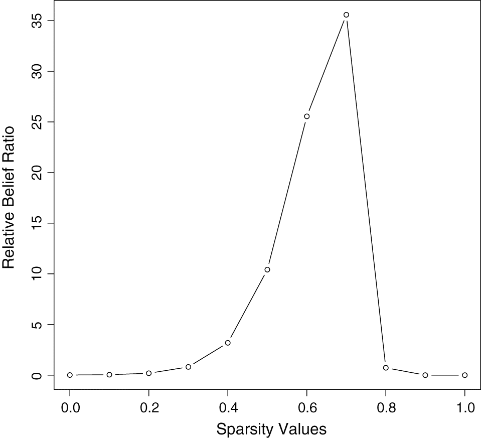
Table 1.
| i | 1 | 2 | 3 | 4 | 5 |
| μi | 0 | 0 | 0 | 0 | 0 |
| RBi(0 | x) | 3.27 | 3.65 | 2.98 | 1.67 | 3.57 |
| Strength | 1.00 | 1.00 | 1.00 | 0.37 | 1.00 |
| i | 6 | 7 | 8 | 9 | 10 |
| μi | 0 | 0 | 2 | 2 | 2 |
| RBi(0 | x) | 3.00 | 3.43 | 2.09 × 10⁻⁴ | 3.99 × 10⁻⁴ | 8.80 × 10⁻³ |
| Strength | 1.00 | 1.00 | 4.25 × 10⁻⁵ | 8.11 × 10⁻⁵ | 1.83 × 10⁻³ |
To investigate sensitivity to the choice of δ several smaller values were considered. Table 2 gives the relevant entries for the same sample as Table 1 when δ = 0.5. The relative belief ratios do not change by much and still give evidence in the right direction. Some of the strengths do change, particularly for i = 1 and i = 6, which now indicate a bit weaker evidence in favor. In this case, ξ(x) = 0.60. Repeating these calculations with δ = 0.1 gives similar results, with the relative belief ratios staying about the same but the strengths getting weaker, and now ξ(x) = 0.50. The insensitivity of the RBi to δ is expected, as the data should increase belief in the interval (μ0 − δ/2, μ0 + δ/2] when H0i is true and decrease it when it is false. It is to be noted, however, that δ is not a tuning parameter of the algorithm but is determined by scientific knowledge in the application as the smallest difference from μ0 of practical importance.
Table 2.
| i | 1 | 2 | 3 | 4 | 5 |
| μi | 0 | 0 | 0 | 0 | 0 |
| RBi(0 | x) | 3.58 | 4.17 | 3.15 | 1.43 | 4.64 |
| Strength | 0.62 | 1.00 | 0.59 | 0.26 | 1.00 |
| i | 6 | 7 | 8 | 9 | 10 |
| μi | 0 | 0 | 2 | 2 | 2 |
| RBi(0 | x) | 3.18 | 3.83 | 3.25 × 10⁻⁵ | 6.76 × 10⁻⁵ | 2.37 × 10⁻³ |
| Strength | 0.59 | 1.00 | 3.30 × 10⁻⁶ | 7.00 × 10⁻⁶ | 2.47 × 10⁻⁴ |
Now, consider basically the same context but with k = 1000, μ1 = … = μ700 = 0 and the remaining μi = 2. In this case, ξ(x) = 0.47, which is a serious underestimate. As such, the multiple testing algorithm will not record enough acceptances and will fail. This problem arises due to the independence of the μi. For the prior distribution of kΞ(θ) is binomial(k, 2Φ(δ/2λ0σ) − 1) and the prior distribution of kϒ(θ) is binomial (k, 2(1 − Φ(δ/2λ0σ))). Thus, the a priori expected proportion of true hypotheses is 2Φ(δ/2λ0σ) − 1 and the expected proportion of false hypotheses is 2(1 − Φ(δ/2λ0σ)). When δ/2λ0σ is small, as when the amount of sampling variability or the diffuseness of the prior are large, then the prior on Ξ suggests a belief in many false hypotheses. When k is small, the data can override this to produce accurate inferences about ξ or υ, but otherwise, large amounts of data are needed that may not be available. Contrary to what is sometimes claimed, testing multiple hypotheses is also a problem in a Bayesian framework.
Example 1 makes it clear that, in general, accurate inference about ξ and υ is not feasible in high-dimensional contexts without large amounts of data. Rather than focus on estimating the proportion of true or false hypotheses, however, we consider an approach designed to protect against false positives or false negatives. It is often the case that when evidence against a hypothesis is obtained it prompts some kind of action, and a user may wish to prevent too many that are spurious. Alternatively, the user may be concerned with too many false negatives, as this may conceal a discovery of real value.
The entries in Tables 1 and 2 point to a feasible approach to these problems by focusing instead on the evidence concerning the individual μi, as these parameters do not depend on high-dimensional aspects of the full model parameter like ξ and υ do. To control the actions taken based on the evidence, constants qR and qA, where 0 < qR ≤ 1 ≤ qA, are used as follows: classify H0i as accepted when RBi(ψ0i | x) > qA and as rejected when RBi(ψ0i | x) < qR. Note that those accepted always have evidence in favor, whereas those rejected always have evidence against. The strengths can also be quoted to assess the reliability of these inferences. Provided qR is greater than the minimum possible value of RBi(⋅ | x), and this is typically 0, and the qA chosen is less than the maximum possible value of RBi(ψ0i | x), and this is 1 over the prior probability of H0i, then this procedure is consistent as the amount of data increases. In fact, the related estimates of ξ and υ are also consistent. The price paid for this is that a hypothesis will not be classified whenever qR ≤ RBi(ψ0i | x) ≤ qA. Not classifying a hypothesis implies that there is not enough evidence for this purpose and more data are required. This approach is referred to as the relative belief multiple testing algorithm.
It remains to determine qA and qR. Consider, first, protecting against too many false positives. The a priori conditional prior probability, given that H0i is true, of finding evidence against H0i less than qR satisfies M(RBi(ψ0i | X) < qR | ψ0i) ≤ qR by Theorem 2. Naturally, we want the probability of a false positive to be small, and choosing qR small accomplishes this. The a priori probability that a randomly selected hypothesis produces a false positive iswhich is bounded above by qR and thus converges to 0 as qR → 0. Also, for fixed qR, eq. (5) converges to 0 as the amount of data increases. More generally qR can be allowed to depend on i, but when the ψi are similar in nature this does not seem necessary. Furthermore, it is not necessary to weight the hypotheses equally, therefore a randomly chosen hypothesis with unequal probabilities could be relevant in certain circumstances. In any case, controlling the value of eq. (5), whether by sample size or by the choice of qR, is clearly controlling for false positives. Suppose there is proportion pFP of false positives that is just tolerable in a problem. Then, qR can be chosen so that eq. (5) is less than or equal to pFP; note that qR = pFP satisfies this.
(5)
Similarly, if then is the prior probability of accepting H0i when is the true value. For a given effect size δ of practical importance it is natural to take . In typical applications this probability decreases the “farther” is from ψ0i, and choosing qA to make this probability small will make it small for all meaningful alternatives. Under these circumstances the a priori probability that a randomly selected hypothesis produces a false negative is bounded above byAs qA → ∞, or as the amount of data increases with qA fixed, then eq. (6) converges to 0 and the number of false negatives can be controlled. If there is proportion pFN of false negatives that is just tolerable in a problem, then qA can be chosen so that eq. (6) is less than or equal to pFN.
(6)
The following optimality result holds for relative belief multiple testing.
Corollary 1: (i) Among all procedures for which the prior probability of accepting H0i, when it is true, is at least M(RBi(ψ0i | X) > qA | ψ0i) for i = 1,…, k, the relative belief multiple testing algorithm minimizes the prior probability that a randomly chosen hypothesis is accepted. (ii) Among all procedures for which the prior probability of rejecting H0i, when it is true, is less than or equal to M(RBi(ψ0i | X) < qR | ψ0i), then the relative belief multiple testing algorithm maximizes the prior probability that a randomly chosen hypothesis is rejected.
Proof: For (i) consider a procedure for multiple testing and let Ai be the set of data values where H0i is accepted. Then, by hypothesis M(RBi(ψ0i | X) > qA | ψ0i) ≤ M(Ai | ψ0i) and by the analog of Theorem 1, M(Ai) ≥ M(RBi(ψ0i | X) > qA). Applying this to a randomly chosen H0i gives the result. The proof of (ii) is basically the same.
Applying the same discussion as after Theorem 1, it is seen that, under reasonable conditions, the relative belief multiple testing algorithm minimizes the prior probability of accepting a randomly chosen H0i when it is false and maximizes the prior probability of rejecting a randomly chosen H0i when it is false. This establishes an optimality result for the relative belief multiple testing algorithm.
Consider now the application of the relative belief multiple testing algorithm in the previous example.
Example 2. Location normal example, continued.
In this context, M(RBi(μ0 | x) < qR | μ0) = 2(1 − Φ(an(qR)) for all i and, therefore, this is the value of eq. (5). Therefore, qR is chosen to make this number suitably small. Table 3 records values for eq. (5) for both the continuous and discretized cases. From this it is seen that for small n there can be some bias against H0i when qR = 1, and thus the prior probability of obtaining false positives is perhaps too large. Table 3 demonstrates that choosing a smaller value of qR can adequately control the prior probability of false positives.
Table 3.
| n | λ0 | qR | (5) | n | λ0 | qR | (5) |
|---|---|---|---|---|---|---|---|
| 1 | 1 | 1 | 0.239 (0.228) | 5 | 1 | 1 | 0.143 (0.097) |
| 1/2 | 0.041 (0.030) | 1/2 | 0.051 (0.022) | ||||
| 1/10 | 0.001 (0.000) | 1/10 | 0.006 (0.001) | ||||
| 2 | 1 | 0.156 (0.146) | 2 | 1 | 0.074 (0.041) | ||
| 1/2 | 0.053 (0.045) | 1/2 | 0.031 (0.013) | ||||
| 1/10 | 0.005 (0.004) | 1/10 | 0.005 (0.001) | ||||
| 10 | 1 | 0.031 (0.026) | 10 | 1 | 0.013 (0.004) | ||
| 1/2 | 0.014 (0.011) | 1/2 | 0.006 (0.002) | ||||
| 1/10 | 0.002 (0.002) | 1/10 | 0.001 (0.001) |
For false negatives, consider eq. (6), wherefor all i. It is easy to show that this is monotone decreasing in δ, and therefore it is an upper bound on the expected proportion of false negatives among those hypotheses that are actually false. The cutoff qA can be chosen to make this number as small as desired. When δ/σ → ∞, then eq. (6) converges to 0 and increases to 2Φ(an(qA)) − 1 as δ/σ → 0. Table 4 records values for eq. (6) when δ/σ = 1 so that the μi differ from μ0 by one half of a standard deviation. There is clearly some improvement but the bias in favor of false negatives is still readily apparent. It would seem that taking gives the best results, but this could be considered s quite conservative. It is also worth remarking that all the entries in Table 4 can be considered very conservative when large effect sizes are expected.
Table 4.
| n | λ0 | qA | (6) | n | λ0 | qA | (6) |
|---|---|---|---|---|---|---|---|
| 1 | 1 | 1.0 | 0.704 (0.715) | 5 | 1 | 1.0 | 0.631 (0.702) |
| 1.2 | 0.527 (0.503) | 2.0 | 0.302 (0.112) | ||||
| 1.4 | 0.141 (0.000) | 2.4 | 0.095 (0.000) | ||||
| 2 | 1.0 | 0.793 (0.805) | 2 | 1.0 | 0.747 (0.822) | ||
| 2.0 | 0.359 (0.304) | 3.0 | 0.411 (0.380) | ||||
| 2.2 | 0.141 (0.000) | 4.5 | 0.084 (0.000) | ||||
| 10 | 1.0 | 0.948 (0.955) | 10 | 1.0 | 0.916 (0.961) | ||
| 5.0 | 0.708 (0.713) | 10.0 | 0.552 (0.588) | ||||
| 10.0 | 0.070 (0.000) | 22.0 | 0.080 (0.000) |
Now, consider the situation when k = 1000, n = 5, δ = 1 and λ0 = 1.94 is the elicited value. From Table 3 with qR = 1.0 about 8% false positives are expected a priori, and from Table 4 with qA = 1.0 a worst case upper bound on the a priori expected percentage of false negatives is about 75%. The top part of Table 5 indicates that with qR = qA = 1.0, then 4.9% (34 of 700) false positives and 0.1% (3 of 300) false negatives were obtained. With these choices of the cutoffs all hypotheses are classified. Certainly the upper bound 75% seems far too pessimistic in light of the results, but recall that Table 4 is computed at the false values μ = ±0.5. The relevant a priori expected percentage of false negatives when μ = ±2.0 is about 3.5%. The bottom part of Table 5 gives the relevant values when qR = 0.5 and qA = 3.0. In this case, there are 2.1% (9 of 428) false positives and 0% false negatives, but 39.9% (272 of 700) of the true hypotheses and 4.3% (13 of 300) of the false hypotheses were not classified as the relevant relative belief ratio lay between qR and qA. Thus, being more conservative has reduced the error rates, but with the drawback that a large proportion of the true hypotheses don’t get classified. The procedure has worked well in this example, but of course the error rates can be expected to rise when the false values move towards the null and improve when they move away from the null.
Table 5.
| Decision | μ = 0 | μ = 2 |
|---|---|---|
| Accept μ = 0 using qA = 1.0 | 666 | 3 |
| Reject μ = 0 using qR = 1.0 | 34 | 297 |
| Not classified | 0 | 0 |
| Accept μ = 0 using qA = 3.0 | 419 | 0 |
| Reject μ = 0 using qR = 0.5 | 9 | 287 |
| Not classified | 272 | 13 |
What is implemented in an application depends on the goals. If the primary purpose is to protect against false positives, then Table 3 indicates that this is accomplished fairly easily. Protecting against false negatives is more difficult; as the actual effect sizes are not known a decision has to be made. Note that choosing a cutoff is equivalent to saying that one will only accept H0i if the belief in the truth of H0i has increased by a factor at least as large as qA. Computations such as those in Table 4 can be used to provide guidance, but there is no avoiding the need to be clear about what effect sizes are deemed to be important or the need to obtain more data when this is necessary. With the relative belief multiple testing algorithm error rates are effectively controlled, but there may be many true hypotheses not classified.
The idea of controlling the prior probability of a randomly chosen hypothesis yielding a false positive or a false negative via eq. (5) or eq. (6), respectively, can be extended. For example, consider the prior probability that a random sample of l from k hypotheses yields at least one false positiveIn the context of the examples in this paper, and many others, the term in eq. (7) corresponding to {i1,…, il} equals M(at least one of for j = 1,…, l | ψ0). The following result leads to an interesting property for eq. (7).
(7)
Lemma 1: Let (Ω, , P) be a probability model and . The probability that at least one of l ≤ k randomly selected events from occurs is increasing in l.
Proof: Let Δ(i) be the event that exactly i of occur, so that ; note that the Δ(i) are mutually disjoint. When l < k,and . Now, consider , which equalsIf l = k, then eq. (8) equals , which is nonnegative. If l < k, then eq. (8) equals , which is nonnegative because an easy calculation shows that each term in the second sum is nonnegative. The expectation of eq. (8) is then nonnegative and this establishes the result.
(8)
It follows, by taking Ai = {x : RBi(ψ0i | x) < qR}, that eq. (7) is an upper bound on the prior probability that a random sample of l′ hypotheses yields at least one false positive whenever l′ ≤ l. Thus, eq. (7) leads to a more rigorous control over the possibility of false positives. A similar result is obtained for false negatives.
Applications
We now consider the sparsity problem.
Example 3. Testing for sparsity.
Consider the context of Example 1. A natural approach to inducing sparsity is to estimate μi by μ0 whenever RBi(μ0 | x) > qA. From the simulation it is seen that this works extremely well when qA = 1 for both k = 10 and k = 1000. It also works when k = 1000 and qA = 3, in the sense that the error rate is low, but it is conservative in the amount of sparsity it induces in that case. Again, the goals of the application will dictate what is appropriate.
Another Bayesian method for inducing sparsity is to use the Bayesian Lasso as per Park and Casella (2008) and based on Tibshirani (1996). The prior here is a product of independent Laplace distributions, namely , where σ is assumed known and μ0, λ0 are hyperparameters. Note that each Laplace prior has mean μ0 and variance . Using the elicitation algorithm provided in Example 1 but replacing the normal prior with a Laplace prior leads to the assignment μ0 = (ml + mu)/2, λ0 = (mu − ml)/2σG−1(0.995), where G−1(p) = 2−1/2 log 2p when p ≤ 1/2, G−1(p) = −2−1/2 log 2(1 − p), where p ≥ 1/2 and G−1 denotes the quantile function of a Laplace distribution with mean 0 and variance 1. With the specifications used in the simulations of Example 1, this leads to μ0 = 0 and λ0 = 1.54, which implies a smaller variance than the value λ0 = 1.94 used with the normal prior, and therefore the Laplace prior is more concentrated about 0.
The posteriors for the μi are independent with the density for μi proportional to giving the MAP estimatorThe MAP estimate of μi is sometimes forced to equal μ0, although this effect is negligible whenever is small.
The Lasso induces sparsity through estimation by taking λ0 to be small. By contrast, the evidential approach, based on the normal prior and the relative belief ratio, induces sparsity through taking λ0 large. The advantage to this latter approach is that by taking λ0 large, prior–data conflict is avoided. When taking λ0 small, the potential for prior–data conflict increases, as the true values can be deep into the tails of the prior. For example, for the simulations of Example 1, , which is smaller than the δ/2 = 0.5 used in the relative belief approach with the normal prior. Therefore, it can be expected that the Lasso will do worse here, and this is reflected in Table 6 in which there are far too many false negatives. To improve this, the value of λ0 needs to be reduced; however, note that this is determined by an elicitation and there is the risk of then encountering prior–data conflict. Another possibility is to implement the evidential approach with the elicited Laplace prior and the discretization as done with the normal prior, and then results similar to those obtained in Example 1 can be expected.
Table 6.
| Decision | μ = 0 | μ = 2 |
|---|---|---|
| Accept μ = 0 using qA = 1.0 | 227 | 0 |
| Reject μ = 0 using qA = 1.0 | 473 | 300 |
It is also interesting to compare the MAP estimation approach and the relative belief approach with respect to the conditional prior probabilities of μi being assigned the value μ0 when the true value actually is μ0. It is easily seen that, based on the Laplace prior, , and this converges to 0 as n → ∞ or λ0 → ∞. For the relative belief approach M(RBi(μ0 | x) > qA | μ0) is the relevant probability. With either the normal or Laplace prior M(RBi(μ0 | x) > qA | μ0) converges to 1 both as n → ∞ and as λ0 → ∞. Therefore, with enough data the correct assignment is always made using relative belief but not with MAP based on the Laplace prior.
The Laplace and normal priors work equally with the relative belief multiple testing algorithm but there are no advantages to using the Laplace prior. One could argue too that the singularity of the Laplace prior at its mode makes it an odd choice and there doesn’t seem to be a good justification for this. Furthermore, the computations are harder with the Laplace prior, particularly with more complex models, and therefore using a normal prior is preferable overall.
An example with considerable practical significance is now considered.
Example 4. Full rank regression.
Suppose the basic model is given by y = β0 + β1x1 + … + βkxk + z = β0 + x′β1:k + z, where the xi are predictor variables, z ∼ N(0, σ2) and β and σ2 are unknown. The problem of interest is testing H0i : βi = 0 for i = 1,…, k to establish which variables have any effect on the response. It is assumed that the observed values of the predictor variable have been standardized so that for observations (y, X) ∈ Rn × Rn×(k+1), where X = (1, x1,…, xk) is of rank k+1, then 1′xi = 0 and ‖xi‖2 = 1 for i = 1,…, k. Note that (b, s), where b = (X′X)−1X′y and s = ‖y − Xb‖, is an MSS for this model, and model checking can be carried out by considering functions of the standardized residuals r = (y − Xb)/s as this has a distribution independent of (β, σ2). The skewness and kurtosis statistics are such functions and it is straightforward to simulate from their distributions to determine if their observed values are surprising.
The prior distribution of (β, σ2) is taken to befor some hyperparameters Σ0 and (α1, α2). Note that this may entail subtracting a known, fixed constant from each y value so that the prior for β0 is centered at 0. Taking 0 as the central value for the priors on the remaining βi seems appropriate when the primary concern is whether or not each xi is having any effect. The marginal prior for βi is then , where t2α1 denotes the t distribution on 2α1 degrees of freedom, for i = 0,…, k. Hereafter, we will take although it is easy to generalize to more complicated choices.
(9)
The elicitation of the hyperparameters is carried out via an extension of a method developed by Cao et al. (2014) for the multivariate normal distribution. Suppose that it is known with virtual certainty, based on our knowledge of the measurements being taken, that β0 + x′β1:k will lie in the interval (−m0, m0) for some m0 > 0 for all x ∈ R, where R is a compact set centered at 0. On account of the standardization, R ⊂ [−1, 1]k. Again “virtual certainty” is interpreted as probability greater than or equal to γ, where γ is some large probability like 0.99. Therefore, the prior on β must satisfy 2Φ(m0/σλ0{1 + x′x}1/2) − 1 ≥ γ for all x ∈ R, and this implies thatwhere with equality when R = [−1, 1]k.
(10)
An interval that will contain a response value y with virtual certainty, given predictor values x, is β0 + x′β1:k ± σz(1+γ)/2. Suppose that we have lower and upper bounds s1 and s2 on the half-length of this interval so that s1 ≤ σz(1+γ)/2 ≤ s2 or, equivalently,holds with virtual certainty. Combining eq. (11) with eq. (10) implies λ0 = m0/s2τ0.
(11)
To obtain the relevant values of α1 and α2 let G(α1, α2,⋅) denote the cdf of the gammarate(α1, α2) distribution, and note that G(α1, α2, z) = G(α1, 1, α2z). Therefore, the interval for 1/σ2 implied by eq. (11) contains 1/σ2 with virtual certainty, when α1, α2 satisfy , or equivalentlyIt is a simple matter to solve these equations for (α1, α2). For this choose an initial value for α1 and, using eq. (12), find z such that G(α1, 1, z) = (1 + γ)/2, which implies . If the left side of eq. (13) is less (or greater) than (1 − γ)/2, then decrease (or increase) the value of α1 and repeat step 1. Continue iterating this process until satisfactory convergence is attained.
(12)
(13)
Evans and Moshonov (2006) showed that when checking for prior–data conflict in such a context it is better to check the components of the prior sequentially as this helps to pinpoint where any failure in the prior occurs. First, the prior on σ2 is checked using the tail probability based on the prior predictive for s and, if this component passes, then the prior on β is checked based on the conditional prior-predictive of b given s. If conflict is found, the methods discussed by Evans and Jang (2011b) are available to modify the prior.
Assuming that X is of rank k+1, the posterior of (β, σ2) is given bywhere and α2(X, y) = ‖y − Xb‖2 + (Xb)′(In − XΣ(X)X′)Xb + 2α2. Then the marginal posterior for βi is given by βi(X, y) + {α2(X, y)σii(X)/(n + 2α1)}1/2tn+2α1 and the relative belief ratio for βi at 0 equals
(14)
(15)
Rather than using eq. (15), however, the distributional results are used to compute the discretized relative belief ratios as in Example 1. For this δ > 0 is required to determine an appropriate discretization and it will be assumed here that this is the same for all the βi, although the procedure can be easily modified if this is not the case in practice. Note that such a δ is effectively determined by the amount that xiβi will vary from 0 for x ∈ R. As xi ∈ [−1, 1], then |xiβi| ≤ δ provided that |βi| ≤ δ. When this variation is suitably small as to be immaterial, then such a δ is appropriate for saying βi is effectively 0. Determination of the hyperparameters and δ is dependent on the application.
Again inference can be made concerning ξ = Ξ(β, σ2), the proportion of the βi effectively equal to 0. As in Example 1, however, we can expect bias when the amount of variability in the data is large relative to δ or the prior is too diffuse. To implement the relative belief multiple testing algorithm, the quantities eqs. (5) and (6) need to be computed to determine qR and qA, respectively. The conditional prior distribution of (b, ‖y − Xb‖2), given (β, σ2), is b ∼ Nk+1(β, σ2(X′X)−1), statistically independent of ‖y − Xb‖2 ∼ gamma((n − k − 1)/2, σ−2/2). Thus, computing eqs. (5) and (6) can be carried out by generating (β, σ2) from the relevant conditional prior, generating (b, ‖y − Xb‖2) given (β, σ2), and using eq. (15).
To illustrate these computations the diabetes data set discussed by Efron et al. (2004) and Park and Casella (2008) is now analyzed. With γ = 0.99, the values m0 = 100, s1 = 75, s2 = 200 were used to determine the prior together with τ0 = 1.05 determined from the X matrix. This led to the values λ0 = 0.48, α1 = 7.29, α2 = 13641.35 being chosen for the hyperparameters. Using the methods developed by Evans and Moshonov (2006), a first check was made on the prior on σ2 against the data, and a tail probability equal to 0.19 was obtained indicating there is no prior–data conflict with this prior. Given no prior–data conflict at the first stage, the prior on β was then checked and the relevant tail probability of 0.00 was obtained indicating a strong degree of conflict. Following the argument of Evans and Jang (2011b), the value of λ0 was increased to choose a prior that was weakly informative with respect to our initial choice. This led to choosing the value λ0 = 5.00, and the relevant tail probability equals 0.32, so there is no conflict.
Using this prior, the relative belief estimates, ratios, and strengths are recorded in Table 7. This shows that there is strong evidence against βi = 0 for the variables sex, bmi, map, and ltg and no evidence against βi = 0 for any other variables. There is strong evidence in favor of βi = 0 for age and ldl, moderate evidence in favor of βi = 0 for the constant, tc, tch, and glu and perhaps only weak evidence in favor of βi = 0 for hdl.
Table 7.
| Variable | Estimates | RBi(0 | X, y) | Strength |
|---|---|---|---|
| Constant | 2 | 2454.86 | 0.44 |
| age | −4 | 153.62 | 0.95 |
| sex | −224 | 0.13 | 0.00 |
| bmi | 511 | 0.00 | 0.00 |
| map | 314 | 0.00 | 0.00 |
| tc | 162 | 33.23 | 0.36 |
| ldl | −20 | 57.65 | 0.90 |
| hdl | 167 | 27.53 | 0.15 |
| tch | 114 | 49.97 | 0.37 |
| ltg | 496 | 0.00 | 0.00 |
| glu | 77 | 66.81 | 0.23 |
As previously discussed, it is necessary to consider the issue of bias, namely to compute the prior probability of getting a false positive for different choices of qR and the prior probability of getting a false negative for different choices of qA. The value of eq. (5) is 0.0003 when qR = 1, and therefore there is virtually no bias in favor of false positives and one can feel confident that the predictors identified as having an effect do so. The story is somewhat different, however, when considering the possibility of false negatives via eq. (6). For example, with qA = 1 then eq. (6) equals 0.9996 and when qA = 100 then eq. (6) equals 0.7998. Thus, there is substantial bias in favor of the null hypotheses and undoubtedly this is due to the diffuseness of the prior. The implication is that we cannot be entirely confident concerning those βi assigned to be equal to 0. Recall that the first prior proposed led to prior–data conflict, and thus a much more diffuse prior obtained by increasing λ0 was substituted. The bias in favor of false negatives with this prior could be reduced by making the prior less diffuse by lowering λ0, but we know that if it is lowered too much prior–data conflict arises. Thus, there is a trade-off between lowering the bias in favor and avoiding prior–data conflict. In any case, determining a value of λ0 in such a fashion seems inappropriate becauase then the prior becomes too dependent on the data and we do not advocate this. The real cure for the bias in an application is to collect more data, and the amount necessary can be determined by the bias calculations.
Next we consider the application to regression with k + 1 > n.
Example 5. Non-full rank regression.
In a number of applications k + 1 > n and thus X is of rank l < n. In this situation, suppose {x1,…, xl} forms a basis for , perhaps after relabeling the predictors, and write X = (1 X1 X2), where X1 = (x1…xl). For given r = (X1 X2)β1:k there will be many solutions β1:k. A particular solution is given by . The set of all solutions is then given by , where , and the columns of C = (−B′ Ik−l)′ give a basis for ker(X1 X2). As sparsity is expected for β1:k, it is natural to consider the solution that minimizes ‖β1:k‖2 for . Using , and applying the Sherman–Morrison–Woodbury formula to C(C′C)−1C′, this is given by the Moore–Penrose solutionwhere ω1:l = (Il + BB′)−1(β1:l + Bβl + 1:k).
(16)
From eq. (9) with , the conditional prior distribution of (β0, ω1:l) given σ2 is , independent of , which, using eq. (16), implies , conditionally independent of β0, whereWith 1/σ2∼ gammarate(α1, α2), this implies that the unconditional prior of the i-th coordinate of is .
Putting gives the full rank model . As in Example 4, then where andNow, noting that (X1 + X2B′)′(X1 + X2B′) = (Il + BB′)X′1X1(Il + BB′), this implies , where is the least-squares estimate of β1:l, andUsing eq. (16), then , independent of , wherewith and . The marginal posterior for is then given by . Relative belief inferences for the coordinates of can now be implemented just as in Example 4.
We consider a numerical example in which there is considerable sparsity. For this let X1 ∈ Rn×l be formed by taking the second through l-th columns of the (l + 1)-dimensional Helmert matrix, repeating each row m times and then normalizing. Thus, n = m(l + 1) and the columns of X1 are orthonormal and orthogonal to 1. It is supposed that the first l1 ≤ l of the variables giving rise to the columns of X1 have βi ≠ 0, whereas the last l − l1 have βi = 0 and that the variables corresponding to the first l2 ≤ k − l columns of X2 = X1B ∈ Rn×(k−l) have βi ≠ 0, whereas the last k − l − l2 have βi = 0. The matrix B is obtained by generating B = diag(B1, B2), where B1 = (z1/‖z1‖…zl2/‖zl2‖) with independent of with IID Nl−l(0, I). Note that this ensures that the columns of X2 are all standardized. Furthermore, because it is assumed that the last l − l1 variables of X1 and the last k − l − l2 variables of X2 don’t have an effect, B is necessarily of the diagonal form given. For, if it was allowed that the last k − l − l2 columns of X2 were linearly dependent on the the first l1 columns of X1, then this would induce a dependence on the corresponding variables, and this is not the intention in the simulation. Similarly, if the first l2 columns of X2 were dependent on the last l − l1 columns of X1, then this would imply that the variables associated with these columns of X1 have an effect, and this is not the intention.
The sampling model is then prescribed by setting l = 10, l1 = 5, l2 = 2, with βi = 4 for i = 1,…, 5, 11, 12 with the remaining βi = 0, σ2 = 1, m = 2, therefore n = 22 and we consider various values of k ≥ l. Note that a different data set was generated for each value of k. The prior is specified as in Example 4, where the values were chosen so that there will be no prior–data conflict arising with the generated data. Also, we considered several values for the discretization parameter δ. A hypothesis was classified as true if the relative belief ratio was >1 and classified as false if it was <1. Table 8 gives the confusion matrices with δ = 0.1. The value δ = 0.5 was also considered, but there was no change in the results.
Table 8.
| k = 10 | Classified positive | Classified negative | Total |
| True positive | 5 | 0 | 5 |
| True negative | 1 | 4 | 5 |
| Total | 6 | 4 | 10 |
| k = 20 | Classified positive | Classified negative | Total |
| True positive | 7 | 0 | 7 |
| True negative | 0 | 13 | 13 |
| Total | 7 | 13 | 20 |
| k = 50 | Classified positive | Classified negative | Total |
| True positive | 7 | 0 | 7 |
| True negative | 0 | 43 | 43 |
| Total | 7 | 43 | 50 |
| k = 100 | Classified positive | Classified negative | Total |
| True positive | 7 | 0 | 7 |
| True negative | 0 | 93 | 93 |
| Total | 7 | 93 | 100 |
One fact stands out immediately, namely that in all of these examples only one misclassification was made and this was in the full rank (k = 10) case where one hypothesis that was true was classified as a positive. The effect sizes that exist are reasonably large, and thus it can’t be expected that the same performance will arise with much smaller effect sizes, but it is clear that the approach is robust to the number of hypotheses considered. It should also be noted, however, that the amount of data is relatively small and the success of the procedure will only improve as this increases. This result can, in part, be attributed to the fact that a logically sound measure of evidence is being used.
Conclusions
The relative belief approach to inference has been applied to problems of practical significance. The central feature is that the inferences are based upon a proper measure of evidence. This approach avoids many of the problems that arise with p-values. For example, there is a natural cutoff to determine when there is either evidence for or against. Given a measure of evidence, a concern with Bayesian methodology can be addressed, namely determining whether or not the ingredients bias the results. Bias calculations play a key role in the multiple testing algorithm and its application to sparsity through the a priori control of false positives and negatives.
There are a number of ingredients that need to be selected to implement the relative belief multiple testing algorithm. Perhaps the most important of these is the model and the most controversial is the prior. For the prior, elicitation algorithms have been provided for each example based on the user being able to specify bounds on parameters that hold with virtual certainty. Given that a measurement process was used in the data collection, this implies restrictions for the values of parameters. For example, suppose interest is in the mean of a response variable corresponding to some kind of length. Each length is measured to a certain accuracy and there is an upper bound on what length can be obtained using a particular measurement technology. Thus, such bounds on the mean response are definitely available and how tight they are depends on what additional information is available on the context. It is also worth noting that there is no reason why some other elicitation algorithm cannot be used if this is felt to be appropriate. There is also the choice of (qR, qA), but these are chosen based on the bias calculations to control for false positives and false negatives and the user will have to select these after considering what proportions of errors are tolerable.
The value of δ in hypothesis assessment problems is seemingly another choice but practical aspects of the measurement process involved in data collection dictate what values make sense. For example, there is no point in considering differences from a mean >0.5 cm if the measurements producing the data are only taken to this accuracy. This provides a lower bound on δ and the application may allow for a larger value. It is comforting, however, that results are reasonably robust to this choice. Determining δ for an arbitrary parameter of interest ψ is not necessarily straightforward, but some guidance, when ψ is a probability and δ is either absolute or relative error, can be found in the work of Al-Labadi et al. (2017).
No mention has been made in the paper concerning the false discovery rate (FDR) approach to multiple testing. Current approaches base this on p-values, but presumably there is no reason why a valid measure of evidence such as the relative belief ratio couldn’t be used instead. It should also be noted that the FDR approach is somewhat different as it does not imply control over both false positive and false negatives, which has been our intent here. The relationship between the approach of this paper and controlling something like the FDR is a topic for further investigation.
Acknowledgements
Michael Evans was supported by a grant from the Natural Sciences and Engineering Research Council of Canada. The authors thank two reviewers for a number of helpful comments.
References
Al-Labadi L, Baskurt Z, and Evans M. 2017. Goodness of fit for the logistic regression model using relative belief. Journal of Statistical Distributions and Applications, 4: 17.
Cao Y, Evans M, and Guttman I. 2014. Bayesian factor analysis via concentration. In Current trends in Bayesian methodology with applications. Edited by SK Upadhyay, U Singh, DK Dey, and A Loganathan. CRC Press, Boca Raton, Florida, USA. pp. 181–201.
Carvalho CM, Polson NG, and Scott JG. 2009. Handling sparsity via the horseshoe. Journal of Machine Learning Research, 5: 73–80.
Efron B, Hastie T, Johnstone I, and Tibshirani R. 2004. Least angle regression. The Annals of Statistics, 32: 407–499.
Evans M. 2015. Measuring statistical evidence using relative belief. Monographs on Statistics and Applied Probability 144. CRC Press, Boca Raton, Florida, USA.
Evans M, and Jang GH. 2011a. A limit result for the prior predictive applied to checking for prior-data conflict. Statistics & Probability Letters, 81: 1034–1038.
Evans M, and Jang GH. 2011b. Weak informativity and the information in one prior relative to another. Statistical Science, 26(3): 423–439.
Evans M, and Moshonov H. 2006. Checking for prior-data conflict. Bayesian Analysis, 1(4): 893–914.
George EI, and McCulloch RE. 1993. Variable selection via Gibbs sampling. Journal of the American Statistical Association, 88: 881–889.
Howson C, and Urbach P. 2006. Scientific reasoning: the Bayesian approach. 3rd edition. Open Court, Chicago, Illinois, USA.
Park R, and Casella G. 2008. The Bayesian Lasso. Journal of the American Statistical Association, 103: 681–686.
Rockova V, and George EI. 2014. EMVS: the EM approach to Bayesian variable selection. Journal of the American Statistical Association, 109(506): 828–846.
Royall R. 1997. Statistical evidence: a likelihood paradigm. Chapman & Hall/CRC Monographs on Statistics & Applied Probability, CRC Press, Boca Raton, Florida, USA.
Rudin W. 1974. Real and complex analysis. 2nd edition. McGraw-Hill, New York, New York, USA.
Salmon W. 1973. Confirmation. Scientific American, 228(5): 75–83.
Strug LJ, and Hodge SE. 2006a. An alternative foundation for the planning and evaluation of linkage analysis. I. Decoupling ‘error probabilities’ from ‘measures of evidence’. Human Heredity, 61: 166–188.
Strug LJ, and Hodge SE. 2006b. An alternative foundation for the planning and evaluation of linkage analysis. II. Implications for multiple test adjustments. Human Heredity, 61: 200–209.
Tibshirani R. 1996. Regression shrinkage and selection via the lasso. Journal of the Royal Statistical Society Series B, 58(1): 267–288.
Information & Authors
Information
Published In

FACETS
Volume 3 • Number 1 • October 2018
Pages: 563 - 583
Editor: Patrick Ingram
History
Received: 20 November 2017
Accepted: 6 February 2018
Version of record online: 25 May 2018
Copyright
© 2018 Evans and Tomal. This work is licensed under a Creative Commons Attribution 4.0 International License (CC BY 4.0), which permits unrestricted use, distribution, and reproduction in any medium, provided the original author(s) and source are credited.
Data Availability Statement
All relevant data are within the paper.
Key Words
Sections
Subjects
Authors
Author Contributions
All conceived and designed the study.
All performed the experiments/collected the data.
All analyzed and interpreted the data.
All contributed resources.
All drafted or revised the manuscript.
Competing Interests
ME is currently serving as a Subject Editor for FACETS, but was not involved in review or editorial decisions regarding this manuscript.
Metrics & Citations
Metrics
Other Metrics
Citations
Cite As
Michael Evans and Jabed Tomal. 2018. Measuring statistical evidence and multiple testing. FACETS.
3(1): 563-583. https://doi.org/10.1139/facets-2017-0121
Export Citations
If you have the appropriate software installed, you can download article citation data to the citation manager of your choice. Simply select your manager software from the list below and click Download.
Cited by
1. Model Checking with Right Censored Data Using Relative Belief Ratio
2. On robustness of the relative belief ratio and the strength of its evidence with respect to the geometric contamination prior
3. The Support Interval
4. Bayesian estimation of extropy and goodness of fit tests
5. Kullback–Leibler divergence for Bayesian nonparametric model checking
6. Measuring and Controlling Bias for Some Bayesian Inferences and the Relation to Frequentist Criteria
7. On one-sample Bayesian tests for the mean