Perspectives from landscape ecology can improve environmental impact assessment
Abstract
The outcomes of environmental impact assessment (EIA) influence millions of hectares of land and can be a contentious process. A vital aspect of an EIA process is consideration of the accumulation of impacts from multiple activities and stressors through a cumulative effects assessment (CEA). An opportunity exists to improve the rigor and utility of CEA and EIA by incorporating core scientific principles of landscape ecology into EIA. With examples from a Canadian context, we explore realistic hypothetical situations demonstrating how integration of core scientific principles could impact EIA outcomes. First, we demonstrate how changing the spatial extent of EIA boundaries can misrepresent cumulative impacts via the exclusion or inclusion of surrounding natural resource development projects. Second, we use network analysis to show how even a seemingly small, localized development project can disrupt regional habitat connectivity. Lastly, we explore the benefits of using long-term historical remote sensing products. Because these approaches are straightforward to implement using publicly available data, they provide sensible opportunities to improve EIA and enhance the monitoring of natural resource development activities in Canada and elsewhere.
Introduction
Despite the cumulative and often widespread impacts of rapid natural resource development (Díaz et al. 2018), management decisions are often made at the level of individual projects. Environmental impact assessment (EIA) is a universally recognized regulatory instrument in environmental management (Morgan 2012) and has remained a consistent—if somewhat contentious—part of natural resource development since its inception in 1970 in the United States (Cashmore 2004; Jay et al. 2007; Morrison-Saunders et al. 2014). Individual project-based EIAs were originally proposed as a regulatory process for identifying, evaluating, and mitigating ecological consequences of development or land use activities. Designated activities that may trigger an EIA vary by jurisdiction but span industries such as forestry, mining, and energy development (Cashmore 2004; Jay et al. 2007). EIA, in some form, is now practiced in nearly all United Nations (UN) member countries (Morgan 2012; Jones 2016). By the 1980s, the further need for cumulative effects assessment (CEA) was recognized because assessing the environmental impact of projects in isolation does not account for combined effects of human activities (Duinker and Greig 2006). Thus, the introduction of CEA (as a sub-field within EIA) expanded EIA to account for multiple stressors over time and space (Jones 2016).
Effective application of CEA within the milieu of EIA has been a persistent challenge. CEA was initially conceived, and is often applied, as an addition to project-based EIA. Yet EIA is limited in its focus on a specific site and set of actions, often accompanied by significant time and resource constraints (Duinker and Greig 2006; Foley et al. 2017; Sinclair et al. 2017). Thus, this need to consider wider spatial and temporal boundaries has resulted in efforts to apply CEA in regional planning and/or strategic level assessments, independent of individual EIA processes (Harriman and Noble 2008; Halseth et al. 2016). Challenges for such broader-scale assessments include limited regulatory support, organizational capacity, weak linkages to other levels of assessment and management decisions, as well as limited data availability (Gunn and Noble 2011; Kristensen et al. 2013; Halseth et al. 2016; Chilima et al. 2017). As the methodology and capacity to implement regional and strategic processes advance (Hodgson and Halpern 2019), and the availability of open data increases, there remains a need to improve the rigour and utility of CEA at the individual project level. Thus, information regarding cumulative impacts remain important for EIA evaluation and decision-making for projects under review (Hegmann and Yarranton 2011; Noble et al. 2017).
A persistent critique has been inadequate integration of high-quality science (particularly ecology) into the practice of CEA–EIA (Morrison-Saunders and Bailey 2003; Morrison-Saunders and Sadler 2010). While acknowledging that strong science is not singularly important to effective and informed decision-making in CEA–EIA, we (and many others) advocate that advancement is needed in this area (Greig and Duinker 2011). Although this call for integration of science into CEA–EIA has been partially answered (via incorporating the science underlying environmental toxicology into technical regulations and guidelines for drinking water and air quality), some scientific realms of ecology remain largely untapped (Hodgson and Halpern 2019). The practice of CEA has not yet widely adopted landscape ecological approaches that utilize a rapidly expanding toolbox of geospatial tools and data products. These opportunities are the focus of this paper, where we aim to not only summarize these challenges, but introduce opportunities for the use of landscape ecology approaches via some illustrative examples. As CEA routinely faces limitations in time, resources, and data (Raudsepp-Hearne and Peterson 2016), the freely available geodata sources routinely used by the landscape ecology community can readily fill data gaps across broad regions and longer time scales.
Spatial and temporal scales of environmental impact assessments
Vital to improving EIA and CEA is defining appropriate spatial and temporal boundaries for assessments. The spatio-temporal scales typically considered in EIA differ from those recommended by ecological research into environmental impacts, as well as differ from best practices for CEA. The spatio-temporal scales of EIA may not be broad enough, or appropriately tailored, to adequately assess the ecological components on which the assessment is focused, especially so for wide-ranging species or regional ecosystem processes (Beanlands and Duinker 1984; Raudsepp-Hearne and Peterson 2016; Venier et al. 2020). The appropriate scales should be defined by the objectives of the research as well as the ecological effects of interest. For instance, habitat connectivity of many wildlife species must be addressed at the landscape scale, whereas soils are better addressed in situ at small scales (Venier et al. 2020).
Although such issues of scale are important throughout an EIA process, some of these scale dilemmas become particularly apparent in the initial scoping stage. Scoping is a fundamental phase of EIA that not only frames the spatio-temporal boundaries of an assessment but also determines which ecological effects/impacts are important to assess. The scoping phase provides a preliminary understanding of how actions (e.g., development, disturbance) will coincide with or impact environmental factors (plants, animals, landscape condition) (Noble 2015). Despite its influence on both EIA and CEA, scoping has been under-researched and is often overlooked (Snell and Cowell 2006). Thus, we explore the impacts of decisions about spatio-temporal scale made in the scoping process and how such decisions can impact subsequent evaluations. Understanding this fundamental influence of scale on our ability to measure and understand environmental response to stressors demonstrates one of the disconnects between ecological science and EIA–CEA (Snell and Cowell 2006).
Defining appropriate spatial and temporal extents for EIA and CEA is a key decision. Yet, this process is fraught with challenges and uncertainties not only due to the complex spatial and temporal dynamics of ecosystem responses and stressors, but also because of the need to combine scientific and participatory perspectives (Squires et al. 2010; Seitz et al. 2011; Ball et al. 2013; Mackinnon et al. 2018). Also challenging is the difficult task of balancing precaution (i.e., including every possible impact and cumulative interaction) with efficiency (i.e., leaving out impacts due to fiscal and/or time constraints) (Mandelik et al. 2005; Snell and Cowell 2006). The spatial extent is often confined to the extent of the particular project under review, rather than in response to ecologically significant boundaries (Seitz et al. 2011; Sinclair et al. 2017). Such deficits have fueled efforts to define ecologically appropriate spatial extents, such as using watersheds as a basis for assessing cumulative impacts to freshwater (Squires et al. 2010; Seitz et al. 2011; Ball et al. 2013). CEA seeks to consider broader temporal scales that include past, present, and reasonably foreseeable future impacts of development beyond those resulting from the specific project under review. Unfortunately, defining appropriate temporal boundaries in EIA and CEA has received limited research attention (Noble 2000; Mackinnon et al. 2018).
The potential role of landscape ecology in improving EIAs
Because of the disconnect between the spatio-temporal scales typically considered in EIA and those recommended by environmental impacts research (Raudsepp-Hearne and Peterson 2016; Venier et al. 2020), we posit that a critical opportunity exists to explicitly consider landscape ecological perspectives, principles, and tools to improve the scientific rigour of CEA–EIA and thus address some of the divide between ecological science and EIA–CEA. Landscape ecology (LE) is an interdisciplinary field focusing on the impacts of disturbance on landscape structure, function, composition, and change. Many of its concepts are centered on the importance of spatial and temporal scale (Liu and Taylor 2002; Turner and Gardner 2015), and the discipline has developed robust and easily accessible methods and tools rooted in real-world applications (Liu and Taylor 2002; Pearson and McAlpine 2010; Gergel and Turner 2017).
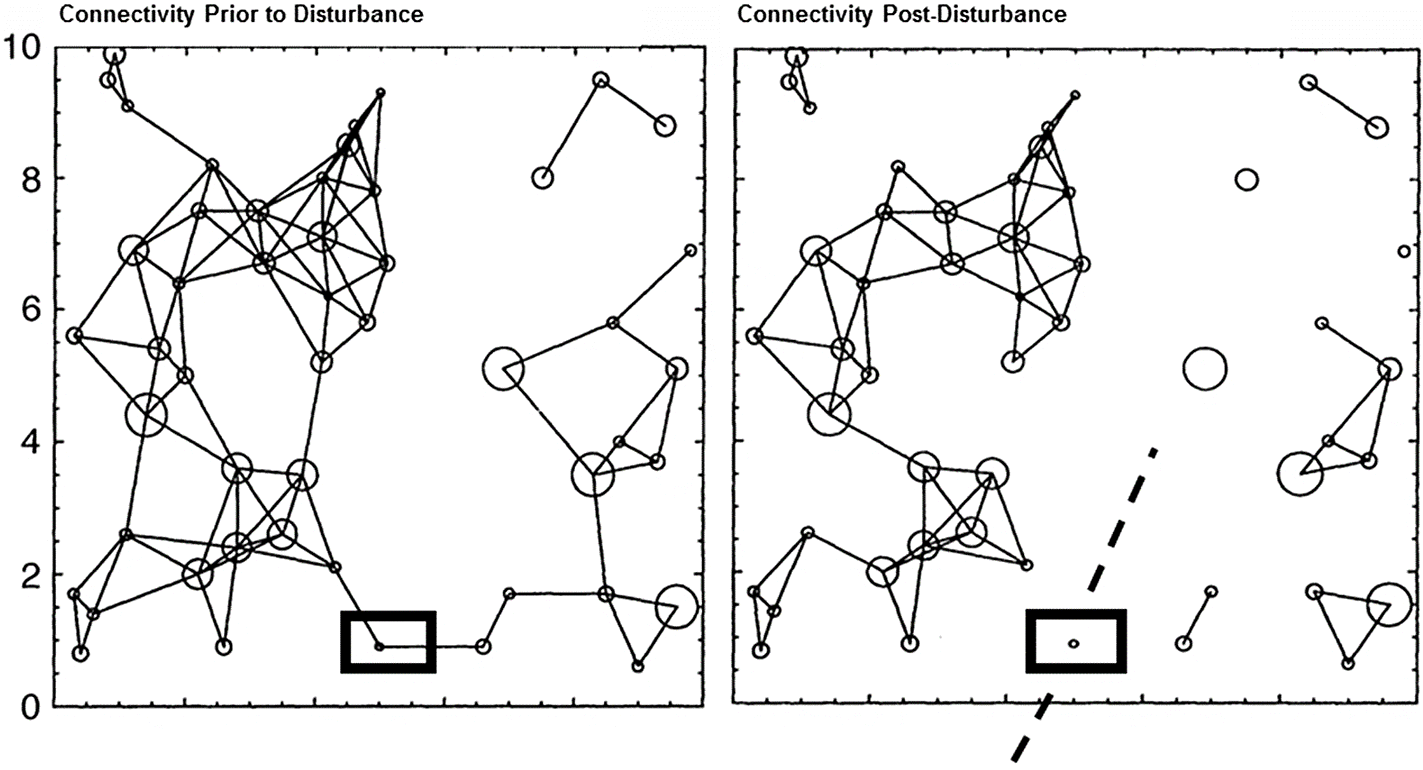
Here, we propose that LE can help us with challenges that have been identified repeatedly by EIA–CEA researchers in terms of defining appropriate spatial and temporal scales for analysis, as well as in providing tools to ground decisions in ecological science. For example, habitat connectivity assessments can be used to help better define ecologically meaningful spatial extents based on species movements or other ecological flows (Tarabon et al. 2019). Methods such as network analysis can detect potentially large changes in connectivity from seemingly small developments (Lookingbill and Minor 2017; Harvey and Altermatt 2019) (Fig. 1). A single project may have little impact on total habitat area when looking exclusively within proposed site boundaries (Fig. 1, left panel). Yet, when viewed within the context of overall landscape connectivity, removal of a quite small area of habitat can greatly reduce overall regional connectivity (Fig. 1, right panel). Such approaches, along with geographic information systems (GIS) and open access remote sensing products, provide information not only useful to local project needs but scalable to broader regional, national, and global-scale analyses (Liu and Taylor 2002; Pearson and McAlpine 2010). Furthermore, the use of long-term archival remote sensing can help augment the temporal extent of analyses.
Fig. 1.
To explore these potential benefits in more depth, we highlight opportunities for LE to be readily integrated into EIA using realistic illustrative examples of natural resource development projects. Although set in British Columbia (BC), Canada, our examples are relevant to advancing the science of EIA’s universally. In Canada, natural resource extraction is widely distributed across its nearly 10 million km2 land base. The areal footprint of resource development in Canada’s boreal alone is expected to increase 50%–60% by 2030 (Price et al. 2013; Webster et al. 2015; Creed et al. 2018; Steenberg et al. 2018). Along with this development comes expansion of vast networks of roads and other linear features (such as seismic lines and pipeline right of ways), which are estimated to account for 80% of boreal anthropogenic disturbance (Pasher et al. 2013). Road development now requires EIAs in many countries (Karlson et al. 2014). However, the quality of EIAs for road projects is generally considered poor because a neglect of cumulative effects may be combined with major uncertainties about the ecological effects of roads (Jaeger 2015; van der Ree et al. 2015). Together, the examples we provide below showcase opportunities to apply LE principles and tools in CEA–EIA assessment.
To demonstrate the application of LE approaches in EIA, we adapt several well-established concepts and tools of LE to provide opportunities for EIA. The first opportunity centers on improving the basis for deciding upon the spatial scale (or extent) of an EIA, with two examples. The second opportunity considers ways to improve EIA using historical information from aerial photography archives to assess baselines over a deeper timeframe. For each opportunity, we begin by introducing key LE concepts, discuss how each concept could enhance the rigour of the EIA process, and then provide example(s) of how the concept could be better integrated into EIA. Recognizing the constraints facing EIA in terms of time, resources, and data (Raudsepp-Hearne and Peterson 2016), we emphasize the accessibility and ease of publicly available “open data” sources along with free and open software. We conclude by elaborating on the ways in which geospatial perspectives can also enhance general monitoring of Canada’s most pressing resource development activities.
Opportunity: improve the rationale underpinning the choice of spatial boundaries
The weighty impact of spatial extent in influencing measurements of ecological processes is a fundamental concept in landscape ecology and in all natural sciences (Turner and Gardner 2015). Similarly, the spatial extent considered in EIA is a complex, context-dependent, and critical decision. Outcomes (particularly for CEA) are inherently shaped by the spatial extent over which they are assessed (João 2002; Karsten et al. 2007; Raudsepp-Hearne and Peterson 2016). Quantifiable, transparent, and repeatable ways to evaluate changes in spatial extent are not routinely used in EIA–CEA. Requirements governing the spatial extent of EIA–CEA are poorly (if at all) defined by legislation in Canada. Thus, decisions about spatial extent can be somewhat arbitrary and often are defined by project proponents (Lebel 2006). Failure to consider the appropriate spatial scale of ecological processes has led to many management failures (i.e., transboundary pollution, vulnerability to flooding events, climate change, population-level fisheries collapses) (Cash et al. 2006). Project-based decision-making, such as EIA approval, is especially susceptible to problems as a result of scale decisions. Although long-term changes are often considered beyond the scope of individual project assessments (Gibson et al. 2016), the accumulation of—and interaction among—stressors from nearby and subsequent developments can create broadscale environmental problems.
In our experience conducting and reviewing EIA scoping procedures, we have not found any standard recommended sizes for use in assessment. Instead, site boundaries are often established and negotiated by proponents on a project-specific basis. For example, BC Environmental Assessment Office (EAO) Guidance outlines several different spatial boundaries to consider (Environmental Assessment Office (EAO) 2013). The different boundary extents include the footprint (i.e., the area of physical works or disturbed ground), the local study area (a larger surrounding area where all or most of the expected effects are to occur), and the regional study area. The regional study area is defined by a natural (watershed, ecological zone) or an artificial boundary (such as a political or economic zone) and are often used to assess cumulative effects. Although consultants use these factors to delineate a spatial boundary, approaches for boundary setting vary by site, industry, and jurisdiction and are often negotiated with economic, social, and political factors in mind.
Next, we explore two examples that demonstrate the implications of the choice of spatial extent on the outcomes of an assessment.
The number and type of developments are influenced by the choice of spatial boundary
In practice, a limiting factor to scaling up local, site-level assessments to a broader spatial extent is often the sheer amount and type of data required (Soranno et al. 2015). However, there has been a strong push within the scientific community to make data more publicly available, combined into larger databases, with more standardized collection efforts. Much of this effort has been enabled by ecological synthesis centers, GIS, and proliferation of big data projects that take advantage of advances in intensive computer processing (Steiniger and Hay 2009; Soranno et al. 2015). Among the most important and widely used open data sources for expanding the spatiotemporal scale of ecological inquiry is archival remote sensing (Kennedy et al. 2010; Frohn and Lopez 2017). Remote sensing is routinely used for a multitude of natural resource applications including tracking land use and land-cover change (Asner and Vitousek 2005) and monitoring anthropogenic and natural disturbances (Gross et al. 2009; Kennedy et al. 2009; Nemani et al. 2009; Kayastha et al. 2012; Thackway et al. 2013). The availability of remote sensing imagery at multiple scales enables multi-scale assessments capable of evaluating the role of spatial extent on perceived impacts.
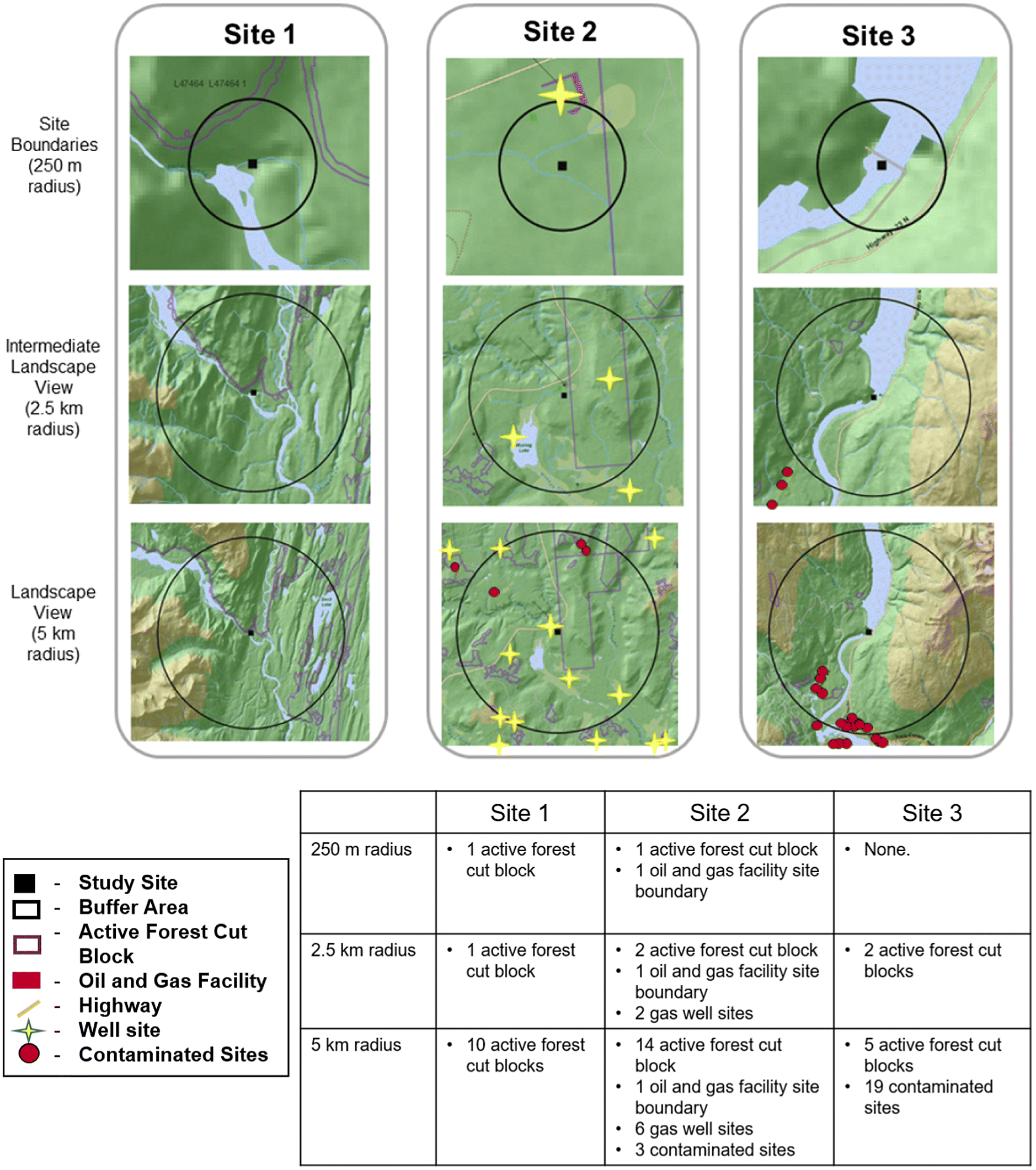
Next, we demonstrate how a multi-scale analysis of potential site boundaries can better characterize outcomes in EIA–CEA. We use a realistic example from the watershed of Skeena River, the only major undammed river in the northern hemisphere (Nilsson et al. 2005; Richardson and Milner 2010). Along with timber extraction since the 1970s, the region is currently facing the highest number of proposed major natural resource development projects in the province (Auditor General of British Columbia 2015), including new mines, liquefied natural gas facilities, crude oil facilities, offshore oil development, as well as hydroelectric projects (Auditor General of British Columbia 2015). From this region, we randomly selected three EIA reviews in the pre-application stage categorized as “Under Review” (using open data from Data BC data.gov.bc.ca/ as of June 2017). For these three projects, we compared the number and type of forest cut blocks (the predominant anthropogenic impact historically) within different radii surrounding the proposed development (Fig. 2). We compared outcomes using 2.5 and 5 km radii because we wanted to comparatively assess the impacts of using different distances for boundary establishment rather than rely on one single arbitrarily chosen extent. Increasing the spatial extent of the study area influenced not only the total number of natural resource development projects but also the type of projects considered (Fig. 2). Thus, the potential cumulative effects associated with any given project can change from few to many with a change in spatial extent. An assessment using only one spatial extent—or solely relying on a small spatial extent—would likely miss a variety of surrounding impacts, thus making a weaker design for CEA.
Fig. 2.
EIA and especially CEA aim to incorporate impacts of past, existing, and reasonable foreseeable developments; thus, landscape context becomes increasingly relevant (Therivel and Ross 2007). Despite CEA’s general goal of evaluating impacts across broader spatial extents, efforts to do so have been limited, in part, because CEA is a requirement for individual project-based EIA. Implementation of such a project-based perspective can result in limited consideration of other nearby projects and of changes over broader spatio-temporal scales (Noble 2015). Furthermore, a lack of regulatory oversight on spatial extent requirements at this stage may allow for the boundaries of the study area to be modified to better suit particular stakeholders (Lebel 2006; Karsten et al. 2007).
We agree that the spatial extent chosen for EIA and CEA should be aligned with the scales over which ecological components operate. But we argue—in addition—that the spatial extent should be a function of other prior, current, and future projects whose proximity or location may interact with the EIA in question. As our example shows, comparisons among different spatial extents can facilitate a richer consideration of cumulative effects from other projects. Although such a requirement to capture a larger spatial extent could be perceived as another roadblock to EIA efficiency, opportunities for landscape-level mitigation, such as restoration of critical habitat lost during past developments, may be revealed. Fortuitously, freely available remote sensing data enables analysis over a variety of spatial extents with little additional effort. To provide transparent and accurate information, the rationale and consequence of choosing a particular spatial extent must be made more explicit in EIA–CEA processes, and analysis spanning multiple extents can provide much-needed context and insight on the implications of scale choices.
Using habitat connectivity networks to help determine appropriate spatial boundaries
Habitat connectivity mapping is another tool for refining the choice of boundaries for project evaluation as they help illustrate the extent over which ecological processes operate and interact. Connectivity refers to the spatial arrangement of land cover (or habitats) and reflects whether movement among patches is facilitated or impeded (Bélisle 2005; Turner and Gardner 2015). Because connectivity is essential for dispersal of individual animals and supporting gene flow among populations, it is fundamental to conservation biology and landscape ecology (Coulon et al. 2004). As such, a wide variety of approaches exist for assessing connectivity ranging from FRAGSTATS (spatial analysis software) to circuit theory and least cost paths (Gergel and Turner 2017). Network analysis adds a further advantage of precisely pinpointing localized impacts that may radiate regionally. Measuring connectivity via network analysis involves a series of “nodes” (or habitat patches) for a particular species of interest which are evaluated relative to their potential links (Urban and Keitt 2001; Kupfer 2012) (Fig. 1). When two nodes are connected through a link, an exchange of energy or material flow is assumed (Urban and Keitt 2001) with important implications for natural resource management.
We used network analysis to evaluate potential changes in landscape-level connectivity from an example proposed project (Fig. 3). We used network analysis to map connectivity of critical habitat for marbled murrelet (Brachyramphus marmoratus), a threatened coastal bird species in the Lakelse Watershed near Terrace, BC (Environment Canada 2014). Suitable habitat was identified using a marbled murrelet suitability model provided by the BC Ministry of Forests, Lands, Natural Resources Operations and Rural Development (BC MFLNRO 2011) based on elevation, distance inland, forest cover, tree height and age, and regional nesting models. Habitat patch sizes and their proximity was then evaluated using CONEFOR connectivity analysis software (Saura and Torné 2009) implemented with an average dispersal distance of 100 m.
Fig. 3.
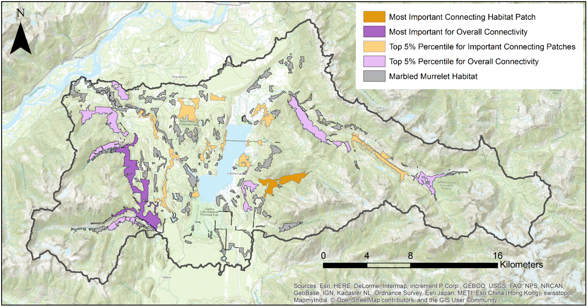
As our example illustrates, conducting a habitat connectivity analysis during EIA can identify situations where projects of relatively limited spatial extent ultimately produce far-reaching impacts on regional connectivity (as in Fig. 1). Although connectivity analyses are often parameterized around a single species, they can also be conducted for multiple species and/or used to infer connectivity changes for general habitats (Venier et al. 2020) such as intact or old-growth habitats. Furthermore, a network analysis can be useful in ranking the importance of specific patches to overall connectivity (Fig. 3) and determine the consequences of losing specific habitat patches (Saura and de la Fuente 2017). Such knowledge of the relative importance of different patches can provide a better understanding of the effects of disturbance and help weigh options for alternative project locations. An evaluation lacking a network analysis might miss far-reaching or disproportionate consequences resulting from a small development.
Ultimately, the spatial extent chosen for EIA and CEA should ultimately be a function of the spatial extent over which affected ecological processes operate (Seitz et al. 2011; Ball et al. 2013; Sinclair et al. 2017). To deepen and operationalize this idea, we further suggest combined use of comparative analyses over multiple extents and network analyses of connectivity for different species, as these approaches provide much-needed guidance for the (albeit imperfect) scaling choices which must be made in EIA–CEA processes.
Opportunity: using historical geospatial information to expand the temporal scale of EIA
Historical landscape ecology has provided many important insights into long-term dynamics of disturbance regimes and ecosystem recovery following disturbance (Swetnam et al. 1999; Higgs et al. 2014), and more recently, long-term responses of ecosystem services following anthropogenic disturbance (Sutherland et al. 2016; Tomscha et al. 2016). Landscape historical approaches particularly shine for determining whether time-lagged responses to disturbance occur (Bürgi et al. 2015; Sutherland et al. 2016). Another key insight of historical ecology is the idea that the typical frame of reference for ecosystem status (e.g., size of a fish stock) for each generation of humanity is different, and often more degraded, than the generation before (Pauly 1995). Often termed shifting baseline syndrome, such perceptions can produce ill-chosen reference points for assessing environmental change (Pauly 1995). Nonetheless, analysis of historical landscapes can help reveal unexpected and complex effects of past policies and decisions shaping landscapes (Higgs et al. 2014; Bürgi et al. 2015; Renard et al. 2015).
In the case of CEA, historical perspectives are important in characterizing past disturbances as well as conditions prior to project development (EAO 2020). However, initial conditions in CEA are often determined using contemporary on-site fieldwork and/or data available over short timespans (i.e., weather monitoring stations, information from nearby projects, etc.). Capturing environmental responses for decision-making requires accurate reference conditions and over scales relevant to the process of interest (Swetnam et al. 1999; Venier et al. 2020), and historical aerial photography can be useful for understanding reference conditions of the deeper past. Availability of historical data is increasing in the current era of big data with growing open-access government data repositories (Wulder et al. 2012; Tomscha et al. 2016).
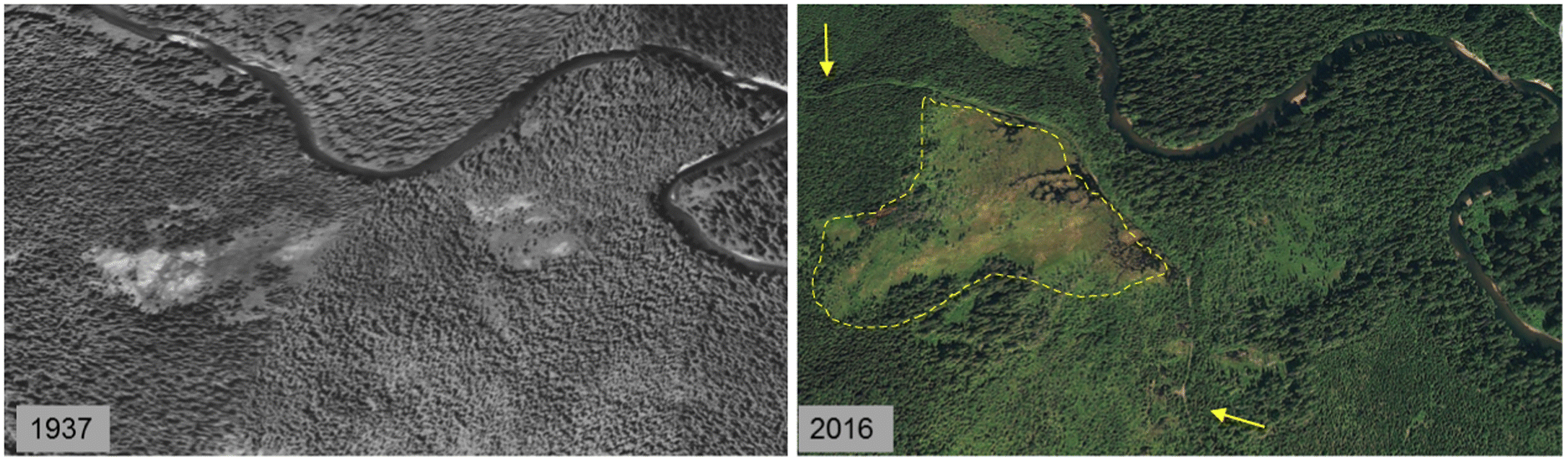
We explored the utility of historical information in EIA–CEA by incorporating historical aerial photography. Despite being somewhat under-utilized for long-term disturbance monitoring (Morgan et al. 2010), aerial photographs exist for much of North America from as early as the 1930s, with more consistent coverage since the 1950s (Morgan and Gergel 2013). Canada’s National Air Photo Library (NAPL) houses one of the world’s most comprehensive archives (exceeding six million photos) dating to the 1920s (NAPL 2020). Using this archival imagery, we examined two situations: changes in floodplain forest composition as well as hydrologic impacts from a forestry road. To do so, we first examined historical vegetation along a 10 km stretch of the Skeena River using Terrestrial Ecosystem Mapping (TEM) protocols (BC Ministry of Environment 2000) based on aerial photographs captured decades apart. Second, we examined a forestry service road along the Lakelse River, a tributary of the Skeena River, taking advantage of early 1937 imagery. To demonstrate the benefits of open data, we used data from BC’s Open Data portal for TEM polygon identification (as completed by de Groot 2005).
Using historical information to improve the evaluation of preconstruction conditions
Integrating historical aerial photos with detailed vegetation information (Fig. 4) can help reconstruct initial landscape conditions prior to development. Historical analysis is a crucial step in learning from past mistakes and ensuring accountability in initial project design, setting reasonable restoration timelines and targets, and increasing the validity of an assessment and subsequent management decisions. Furthermore, the idea offers potential for project proponents to reduce cumulative effects by restoring previously degraded ecosystems as part of mitigation, restoration, or decommissioning of a contemporary project. We recommend developing a more rigorous process for characterizing historical ecosystems whereby the temporal scale considered includes deeper information about past pressures using historical geodata. Application of this approach in a CEA–EIA context would support a much deeper consideration of the temporal range used in assessments.
Fig. 4.

Historical aerial photography can improve our understanding of the long-term impacts of roads
Another common challenge in EIA is the need to explicitly account for roads and road building during resource extraction. Despite their narrow spatial footprint (in comparison to disturbances such as clear-cutting), road impacts can be quite varied, persistent, and manifest at landscape scales (Venier et al. 2020). Impacts can range from habitat loss and fragmentation for both aquatic and terrestrial biodiversity, spread of invasive species, altered predator–prey dynamics, sedimentation, tree mortality, and disruption of hydrological connectivity in wetlands (Trombulak and Frissell 2000; Eigenbrod et al. 2009; Williams et al. 2013). Historical road construction, in particular, caused compaction and altered drainage patterns (Young et al. 2017). Despite the improved design of modern culverts, road construction can still impact natural drainage when blocked by sediment or beaver dams or when installed in inappropriate locations (Mader 2014; Bocking et al. 2017). As such, CEA should give careful consideration of road placement with a view to historical practices—together with adjacent and future road construction—to inform assessment of cumulative effects.
Historical road construction and its long-term impact on nearby wetlands can be visually assessed using freely available historical aerial photography archives (Fig. 5), reaching back to a view that is decades earlier than typical preconstruction field surveys. When roads alter natural drainage patterns and reduce hydrological connectivity, both desiccation and flooding can result. Patterns of both flooding and dessication are visible in Fig. 5, which exemplifies the persistent effects of past roads on the landscape, with impacts lasting long after construction (Webster et al. 2015). This legacy is particularly severe for older roads, often originally built with improper placement, insufficient mitigation, and/or overall more intrusive construction practices. Thus, it’s important to ground contemporary assessments with knowledge of past historical practices. We argue that understanding the long-term hydrologic impacts of roads is critical and that historical information can improve this understanding. The persistent long-term legacy of road impacts may be missed without an evaluation of historical imagery for a project location. If CEA–EIA processes do not incorporate impacts of past road building within the context of past construction practices, a full accounting of cumulative impacts cannot be achieved.
Fig. 5.
Implications
Expanding the spatio-temporal scale of EIA–CEA with remote sensing
One of the persistent challenges in EIA is collecting sufficient data to match the temporal scale of impacts. To delve even deeper into the past, aerial photography is notable in that it represents the longest spatially contiguous historic imagery of earth’s surface, generally dating back to the 1950s (or even earlier) in many places (Morgan et al. 2010). As such, it has been used for decades to characterize forests and wetland vegetation (Frayer et al. 1983; Hardisky and Klemas 1983; Tiner et al. 2015). Historical aerial photography can fill in data gaps and characterize vegetative–wetland trends in data-limited or hard to access areas. As such, aerial photos and satellite imagery have been used in both Canada and the United States to create the Canadian Wetland Inventory (Ducks Unlimited 2018) and the National Wetlands Inventory, respectively (Dahl and Watmough 2007). Air photos and historical imagery are commonly used for site assessments of contaminated sites and in remediation plans (commonly referred to as Phase I Environmental Assessments or Preliminary Site Investigations) to uncover previous uses of a site. Yet the use of air photos and historical imagery is not common in the scoping stages of EIA, suggesting that although such resources are available, they are under-utilized by practitioners.
A fundamental trade-off exists between image resolution (which affects discernable detail) and image processing time and cost (Frohn and Lopez 2017). For example, aerial photography is often acquired at very high spatial resolution yet may require substantial time for processing and interpretation over vast areas (Morgan et al. 2010). In contrast, lower spatial resolution satellites, such as MODIS, provide broader spatial coverage (at regional to global spatial scales) and twice-daily temporal resolution at no cost, yet are unable to detect fine-scale ecological patterns (Potter et al. 2016).
Landsat imagery provides a useful compromise among the trade-offs in scale and cost (Cohen and Goward 2004; Wulder et al. 2012, 2016). The opening of the Landsat archive for public use by the United States Geological Survey in 2008 (Woodcock et al. 2008) has further revolutionized its utility. With over 40 years of observations at a medium resolution (30 m) and ∼16-d intervals for parts of the world, this expansion of spatial and temporal coverage has supported an exponential increase in the scientific use of Landsat imagery (Wulder et al. 2012). Building on this, recent advancements for Canada include a nationwide Best Available Pixel Landsat database (White and Wulder 2014; Hermosilla et al. 2016), fulfilling the need for free and open data in a “user-ready” database. As open data become increasingly accessible to scientists at academic institutions, government agencies, and consulting companies, there will be greater opportunity to improve landscape monitoring and bolster landscape-level decision-making in natural resource developments, particularly EIA–CEA. Some of the greatest opportunities to exploit the utility and benefits of open remote sensing data will likely transpire in historically understudied and inaccessible landscapes, such as those found throughout the vast extent of northern Canada.
When used in tandem, the combination of aerial photography and Landsat provide an unparalleled opportunity to assess landscapes at high spatial resolution, over a variety of spatial extents, over longer time frames, and evaluate the impacts of activities causing land cover change. Because the use of air photos and remote sensing has potential to fill in data gaps in different ways, one of the goals of landscape analysts should be to better integrate historical photography and long-term satellite archives to improve the assessment of changing landscape connectivity across different spatial extents in EIA and CEA.
Conclusions
The rapid pace and broad scale of development often exceeds our ability to monitor, much less understand, its environmental impact. Contending with environmental change, especially in remote areas throughout Canada, will require data acquisition and analysis methods with relevance for examining understudied systems over broad spatio-temporal extents (Soranno et al. 2015). Empirical data and new methods are required for robust EIA development and decision-making. The expanding availability of geodata provides new opportunities for EIA, CEA, and monitoring. Combining smaller site-level assessments using aerial photos with imagery from satellite remote sensing provides an important way forward. When combined with perspectives on scaling and landscape history from the discipline of landscape ecology, remote sensing can improve the spatio-temporal context for assessing cumulative impacts and stressors.
Through a series of examples, we have demonstrated how landscape ecology concepts (varying spatial extents), tools (connectivity analysis), and data sources (historical imagery) can contribute to advancing the scientific rigour of CEA. We conclude that the choices made regarding spatial extent in CEA can be better informed through using comparative analyses over multiple extents and network analyses of connectivity. The temporal range of assessments should also include historical road construction and effects on wetlands. All these examples follow relatively simple LE methods, which we believe can be readily adopted to improve the scientific rigour of CEA. With an array of tools that are easily implementable, and have a defensible foundation in the scientific literature, landscape ecology can provide improved information for regulators, decision-makers, and resource managers, and more accurately account for the impacts and benefits of development.
Although the potential for geospatial researchers to participate in policy has been lauded (Mayer and Lopez 2011), often such participation has not been well-linked to policy specifics (De Leeuw et al. 2010). Despite successful implementation of remote sensing into some aspects of policy (such as satellite detection of the ozone-layer hole which culminated in a chlorofluorocarbon ban), remote sensing is under-utilized to answer specific policy questions and evaluate policy outcomes. In the past, barriers to the use of landscape and remote sensing analysis included cost, specialized skill, lack of data and software, inconsistent methods, and fluctuating political reasons (Mayer and Lopez 2011). Along with the markedly declining costs of imagery, open access data products are now increasingly “user-ready,” with image preprocessing already complete. With geodata such as the National Land Cover Database (Homer et al. 2020) and Best-Available Pixel (White and Wulder 2014), specialized skills for preprocessing and classification of raw imagery no longer present problems. Countries are also implementing coordinated transborder classification systems such as the CORINE database spanning most of Europe (EEA 2020). Specialized skills are also becoming more widely accessible through open access Landscape Ecology MOOCs (edx.org/course/landscape-ecology), course-based Masters programs in geomatics, and textbooks with shareware resources (Gergel and Turner 2017). Participatory mapping methods (which can help directly address resource use concerns of local communities) is also being increasingly linked to remote sensing, providing further avenues to foster links between remote sensing, policy, and public perception of landscape disruption (Eddy et al. 2017).
As these conceptual and technical barriers continue to crumble, future landscape ecological research should focus on making more direct links to policy development, policy implementation, and policy evaluation to utilize the full potential of such expanding technology. More robust, transparent, and routine integration of remote sensing into EIA will help promote the validity of EIA work and enhance public confidence in the assessment, review, and approval process. The conceptual approaches of landscape ecology provide useful insights into improving EIA and are primed to help build better connections between scientific research, EIA practice, and decision-making.
Acknowledgements
KJH was supported by an NSERC CGS-Master’s scholarship, UBC Forestry’s Strategic Recruitment Fund, the NSERC Canadian Network of Aquatic Ecosystem Services, World Wildlife Fund (WWF)—Canada as well as an NSERC Discovery Grant to SEG. We would also like to thank James Casey of WWF-Canada for his role as a catalyst in this work.
References
Asner GP, and Vitousek PM. 2005. Remote analysis of biological invasion and biogeochemical change. Proceedings of the National Academy of Sciences of the United States of America, 102(12): 4383–4386.
Auditor General of British Columbia. 2015. Managing the cumulative effects of natural resource development in B.C. [online]: Available from bcauditor.com/sites/default/files/publications/reports/OAGBC%20Cumulative%20Effects%20FINAL.pdf.
Ball M, Noble BF, and Dubé MG. 2013. Valued ecosystem components for watershed cumulative effects: an analysis of environmental impact assessments in the South Saskatchewan River watershed, Canada. Integrated Environmental Assessment and Management, 9(3): 469–479.
BC Ministry of Environment. 2000. [online]: Available from www2.gov.bc.ca/assets/gov/environment/natural-resource-stewardship/nr-laws-policy/risc/tem_man.pdf.
Beanlands GE, and Duinker PN. 1984. An ecological framework for environmental impact assessment. Journal of Environmental Management, 18(3): 267–277.
Bélisle M. 2005. Measuring landscape connectivity: the challenge of behavioral landscape ecology. Ecology, 86: 1988–1995.
Bocking E, Cooper DJ, and Price J. 2017. Using tree ring analysis to determine impacts of a road on a boreal peatland. Forest Ecology and Management, 404: 24–30.
British Columbia Ministry of Forests, Lands, Natural Resource Operations and Rural Development (BC MFLNRO). 2011. Marbled murrelet habitat suitability model [online]: Available from catalogue.data.gov.bc.ca/dataset/marbled-murrelet-suitability-model.
Bürgi M, Silbernagel J, Wu J, and Kienast F. 2015. Linking ecosystem services with landscape history. Landscape Ecology, 30: 11–20.
Cash DW, Adger WN, Berkes F, Garden P, Lebel L, Olsson P, et al. 2006. Scale and cross-scale dynamics: governance and information in a multilevel world. Ecology and Society, 11(2): 8.
Cashmore M. 2004. The role of science in environmental impact assessment: process and procedure versus purpose in the development of theory. Environmental Impact Assessment Review, 24: 403–426.
Chilima JS, Blakely JAE, Noble BF, and Patrick RJ. 2017. Institutional arrangements for assessing and managing cumulative effects on watersheds: lessons from the Grand River watershed, Ontario, Canada. Canadian Water Resources Journal, 42(3): 223–236.
Cohen WB, and Goward SN. 2004. Landsat’s role in ecological applications of remote sensing. BioScience, 54(6): 535–545.
Coulon A, Cosson JF, Angibault JM, Cargnelutti B, Galan M, Morellet N, et al. 2004. Landscape connectivity influences gene flow in a roe deer population inhabiting a fragmented landscape: an individual-based approach. Molecular Ecology, 13: 2841–2850.
Creed IF, Duinker PN, Steenberg JWN, and Serran JN. 2018. Managing risks to Canada’s boreal zone: transdisciplinary thinking in pursuit of energy security. Environmental Reviews, 27(3): 407–418.
Dahl TE, and Watmough MD. 2007. Current approaches to wetland status and trends monitoring in prairie Canada and the continental United States of America. Canadian Journal of Remote Sensing, 33: S17–S27.
de Groot A. 2005. Review of the hydrology, geomorphology, ecology and management of the Skeena River floodplain. Bulkley Valley Research Centre.
De Leeuw J, Georgiadou Y, Kerle N, De Gier A, Inoue Y, Ferwerda J, et al. 2010. The function of remote sensing in support of environmental policy. Remote Sensing, 2(7): 1731–1750.
Díaz S, Pascual U, Stenseke M, Martín-López B, Watson RT, Molnár Z, et al. 2018. Assessing nature’s contributions to people. Science, 359(6373): 270–272.
Ducks Unlimited. 2018. Canadian Wetland Inventory [online]: Available from ducks.ca/initiatives/canadian-wetland-inventory/.
Duinker PN, and Greig LA. 2006. The impotence of cumulative effects assessment in Canada: ailments and ideas for redeployment. Environmental Management, 37(2): 153–161.
Eddy IMS, Gergel SE, Coops NC, Henebry GM, Levine J, Zerriffi H, et al. 2017. Integrating remote sensing and local ecological knowledge to monitor rangeland dynamics. Ecological Indicators, 82: 106–116.
Eigenbrod F, Hecnar SJ, and Fahrig L. 2009. Quantifying the road-effect zone: threshold effects of a motorway on anuran populations in Ontario, Canada. Ecology and Society, 14(1): 24.
Environment Canada. 2014. Recovery strategy for the marbled murrelet (Brachyramphus marmoratus) in Canada. Species at Risk Act Recovery Strategy Series. Environment Canada, Ottawa, Ontario. v + 49 p.
Environmental Assessment Office (EAO). 2013. Guideline for the selection of valued components and assessment of potential effects [online]: Available from www2.gov.bc.ca/assets/gov/environment/natural-resource-stewardship/environmental-assessments/guidance-documents/eao-guidance-selection-of-valued-components.pdf.
Environmental Assessment Office (EAO). 2020. EAO user guide [online]: Available from www2.gov.bc.ca/assets/gov/environment/natural-resource-stewardship/environmental-assessments/guidance-documents/2018-act/eao_user_guide_v101.pdf.
European Environment Agency (EEA). 2020. European Union, Copernicus land monitoring service.
Foley MM, Mease LA, Martone RG, Prahler EE, Morrison TH, Murray CC, et al. 2017. The challenges and opportunities in cumulative effects assessment. Environmental Impact Assessment Review, 62: 122–134.
Frayer WE, Monahan TJ, Bowden DC, and Graybill FA. 1983. Status and trends of wetlands and deepwater habitats in the conterminous United States, 1950’s to 1970’s.
Frohn RC, and Lopez RD. 2017. Remote sensing for landscape ecology: new metric indicators: monitoring, modeling, and assessment of ecosystems. CRC Press.
Gergel SE, and Turner MG (Editors). 2017. Learning landscape ecology: a practical guide to concepts and techniques. 2nd edition. Springer, New York, New York. 347 p.
Gibson RB, Doelle M, and Sinclair AJ. 2016. Fulfilling the promise: basic components of next generation environmental assessment. Journal of Environmental Law and Practice, 29: 257–283.
Greig LA, and Duinker PN. 2011. A proposal for further strengthening science in environmental impact assessment in Canada. Impact Assessment and Project Appraisal, 29: 159–165.
Gross JE, Goetz SJ, and Cihlar J. 2009. Application of remote sensing to parks and protected area monitoring: introduction to the special issue. Remote Sensing of Environment, 113(7): 1343–1345.
Gunn J, and Noble BF. 2011. Conceptual and methodological challenges to integrating SEA and cumulative effects assessment. Environmental Impact Assessment Review, 31(2): 154–160.
Halseth GR, Gillingham MP, Johnson CJ, and Parkes MW. 2016. Cumulative effects and impacts: the need for a more inclusive, integrative, regional approach. In Integration imperative: cumulative environmental, community and health effects of multiple natural resource developments. Edited by MP Gillingham, GR Halseth, CJ Johnson, and MW Parkes. Springer International Publishing, Cham, Switzerland. pp. 3–21.
Hardisky MA, and Klemas V. 1983. Tidal wetlands natural and human-made changes from 1973 to 1979 in Delaware: mapping techniques and results. Environmental Management, 7(4): 339–344.
Harvey E, and Altermatt F. 2019. Regulation of the functional structure of aquatic communities across spatial scales in a major river network. Ecology, 100(4): e02633.
Hegmann G, and Yarranton GA. 2011. Alchemy to reason: effective use of cumulative effects assessment in resource management. Environmental Impact Assessment Review, 31(5): 484–490.
Hermosilla T, Wulder MA, White JC, Coops NC, Hobart GW, and Campbell LB. 2016. Mass data processing of time series Landsat imagery: pixels to data products for forest monitoring. International Journal of Digital Earth, 9(11): 1035–1054.
Higgs E, Falk DA, Guerrini A, Hall M, Harris J, Hobbs RJ, et al. 2014. The changing role of history in restoration ecology. Frontiers in Ecology and the Environment, 12: 499–506.
Hodgson EE, and Halpern BS. 2019. Investigating cumulative effects across ecological scales. Conservation Biology, 33(1): 22–32.
Homer C, Dewitz J, Jin S, Xian G, Costello C, Danielson P, et al. 2020. Conterminous United States land cover change patterns 2001–2016 from the 2016 National Land Cover Database. ISPRS Journal of Photogrammetry and Remote Sensing, 162: 184–199.
Jaeger JAG. 2015. Improving environmental impact assessment and road planning at the landscape scale. In Handbook of road ecology. Edited by R van der Ree, DJ Smith, and C Grilo. John Wiley & Sons, Ltd. pp. 32–42.
Jay JS, Slinn P, and Wood C. 2007. Environmental impact assessment: retrospect and prospect. Environmental Impact Assessment Review, 27: 287–300.
João E. 2002. How scale affects environmental impact assessment. Environmental Impact Assessment Review, 22: 289–310.
Jones FC. 2016. Cumulative effects assessment: theoretical underpinnings and big problems. Environmental Reviews, 24: 187–204.
Karlson M, Mörtberg U, and Balfors B. 2014. Road ecology in environmental impact assessment. Environmental Impact Assessment Review, 48: 10–19.
Karsten SA, Bots PW, and Slinger JH. 2007. Spatial boundary choice and the views of different actors. Environmental Impact Assessment Review, 27: 386–407.
Kayastha N, Thomas V, Galbraith J, and Banskota A. 2012. Monitoring wetland change using inter-annual landsat time-series data. Wetlands, 32(6): 1149–1162.
Kennedy RE, Townsend PA, Gross JE, Cohen WB, Bolstad P, Wang YQ, et al. 2009. Remote sensing change detection tools for natural resource managers: understanding concepts and tradeoffs in the design of landscape monitoring projects. Remote Sensing of Environment, 113(7): 1382–1396.
Kennedy RE, Yang Z, and Cohen WB. 2010. Detecting trends in forest disturbance and recovery using yearly landsat time series: 1. LandTrendr—temporal segmentation algorithms. Remote Sensing of Environment, 114(12): 2897–2910.
Kristensen S, Noble BF, and Patrick RJ. 2013. Capacity for watershed cumulative effects assessment and management: lessons from the lower fraser river basin, Canada. Environmental Management, 52(2): 360–373.
Kupfer JA. 2012. Landscape ecology and biogeography: rethinking landscape metrics in a post FRAGSTATS landscape. Progress in Physical Geography, 36: 400–420.
Lebel L. 2006. The politics of scale in environmental assessment. In Bridging scales and knowledge systems: concepts and applications in ecosystem assessment. Edited by WV Reid, F Berkes, T Wilbanks, and D Capistrano. Island Press, Washington, D.C. pp. 37–57.
Liu J, and Taylor W. 2002. Integrating landscape ecology into natural resource management. Cambridge University Press, New York, New York.
Lookingbill T, and Minor E. 2017. Assessing multi-scale landscape connectivity using network analysis. Chapter 12. In Learning landscape ecology: a practical guide to concepts and techniques. 2nd edition. Edited by SE Gergel and MG Turner. Springer, New York, New York.
Mackinnon AJ, Duinker PN, and Walker TR. 2018. The application of science in environmental impact assessment. Routledge Focus on Environment and Sustainability. Taylor & Francis Group, London, UK. 141 p.
Mader K. 2014. Mitigating impacts of new forest access roads on water levels in forested wetlands: are cross-drains enough? Master’s thesis, Dalhousie University, Halifax, Nova Scotia.
Mandelik Y, Dayan T, and Feitelson E. 2005. Issues and dilemmas in ecological scoping: scientific, procedural and economic perspectives. Impact Assessment and Project Appraisal, 23: 55–63.
Mayer AL, and Lopez RD. 2011. Use of remote sensing to support forest and wetlands policies in the USA. Remote Sensing, 3(6): 1211–1233.
Morgan JL, and Gergel SE. 2013. Automated analysis of aerial photographs and potential for historic forest mapping. Canadian Journal of Forest Research, 43(8): 699–710.
Morgan JL, Gergel SE, and Coops NC. 2010. Aerial photography: a rapidly evolving tool for ecological management. BioScience, 60: 47–59.
Morgan RK. 2012. Environmental impact assessment: the state of the art. Impact Assessment and Project Appraisal, 30: 5–14.
Morrison-Saunders A, and Bailey J. 2003. Practitioner perspectives on the role of science in environmental impact assessment. Environmental Management, 31: 683–695.
Morrison-Saunders A, and Sadler B. 2010. The art and science of impact assessment: results of a survey of IAIA members. Impact Assessment and Project Appraisal, 28: 77–82.
Morrison-Saunders A, Pope J, Gunn JA, Bond A, and Retief F. 2014. Strengthening impact assessment: a call for integration and focus. Impact Assessment and Project Appraisal, 32: 2–8.
National Air Photo Library (NAPL). 2020 [online]: Available from nrcan.gc.ca/maps-tools-publications/satellite-imagery-air-photos/air-photos/22030.
Nemani R, Hashimoto H, Votava P, Melton F, Wang W, Michaelis A, et al. 2009. Monitoring and forecasting ecosystem dynamics using the Terrestrial Observation and Prediction System (TOPS). Remote Sensing of Environment, 113(7): 1497–1509.
Nilsson C, Reidy CA, Dynesius M, and Revenga C. 2005. Fragmentation and flow regulation of the world’s large river systems. Science, 308(5720): 405–408.
Noble B, Liu J, and Hackett P. 2017. The contribution of project environmental assessment to assessing and managing cumulative effects: individually and collectively insignificant? Environmental Management, 59(4): 531–545.
Noble BF. 2000. Strengthening EIA through adaptive management: a systems perspective. Environmental Impact Assessment Review, 20(1): 97–111.
Noble BF. 2015. Introduction to environmental impact assessment: a guide to principles and practice. Oxford University Press, Don Mills, Ontario.
Pasher J, Seed E, and Duffe J. 2013. Development of boreal ecosystem anthropogenic disturbance layers for Canada based on 2008 to 2010 Landsat imagery. Canadian Journal of Remote Sensing, 39(1): 42–58.
Pauly D. 1995. Anecdotes and the shifting baseline syndrome of fisheries. Trends in Ecology & Evolution, 10: 430.
Pearson DM, and McAlpine CA. 2010. Landscape ecology: an integrated science for sustainability in a changing world. Landscape Ecology, 25: 1151–1154.
Potter KM, Koch FH, Oswalt CM, and Iannone BV. 2016. Data, data everywhere: detecting spatial patterns in fine-scale ecological information collected across a continent. Landscape Ecology, 31(1): 67–84.
Price DT, Alfaro RI, Brown KJ, Flannigan MD, Fleming RA, Hogg EH, et al. 2013. Anticipating the consequences of climate change for Canada’s boreal forest ecosystems. Environmental Reviews, 21: 322–365.
Raudsepp-Hearne C, and Peterson GD. 2016. Scale and ecosystem services: how do observation, management, and analysis shift with scale—lessons from Québec. Ecology and Society, 21(3): 16.
Renard D, Rhemtulla JM, and Bennett EM. 2015. Historical dynamics in ecosystem service bundles. Proceedings of the National Academy of Sciences of the United States of America, 112: 13411–13416.
Richardson JS, and Milner AM. 2010. Chapter 16. Pacific Coast Rivers (Canada and Alaska). In Field guide to rivers of North America. Edited by AC Benke and CE Cushing. Elsevier, Burlington, Massachusetts. pp. 320–341.
Saura S, and de la Fuente B. 2017. Advances in quantifying habitat connectivity using graph theory (with Conefor). Chapter 14. In Learning landscape ecology: a practical guide to concepts and techniques. 2nd edition. Edited by SE Gergel and MG Turner. Springer, New York, New York.
Saura S, and Torné J. 2009. Conefor Sensinode 2.2: a software package for quantifying the importance of habitat patches for landscape connectivity. Environmental Modelling & Software, 24(1): 135–139.
Seitz NE, Westbrook CJ, and Noble BF. 2011. Bringing science into river systems cumulative effects assessment practice. Environmental Impact Assessment Review, 31(3): 172–179.
Sinclair AJ, Doelle M, and Duinker PN. 2017. Looking up, down, and sideways: reconceiving cumulative effects assessment as a mindset. Environmental Impact Assessment Review, 62: 183–194.
Snell T, and Cowell R. 2006. Scoping in environmental impact assessment: balancing precaution and efficiency? Environmental Impact Assessment Review, 26: 359–376.
Soranno PA, Bissell EG, Cheruvelil KS, Christel ST, Collins SM, Fergus CE, et al. 2015. Building a multi-scaled geospatial temporal ecology database from disparate data sources: fostering open science and data reuse. Gigascience, 4: 28.
Squires AJ, Westbrook CJ, and Dubé MG. 2010. An approach for assessing cumulative effects in a model river, the Athabasca River basin. Integrated Environmental Assessment and Management, 6(1): 119–134.
Steenberg JWN, Duinker PN, Creed IF, Serran JN, and Ouellet Dallaire C. 2018. Alternative scenarios for the future of the Canadian boreal zone. Environmental Reviews, 27(2): 185–199.
Steiniger S, and Hay GJ. 2009. Free and open source geographic information tools for landscape ecology. Ecological Informatics, 4(4): 183–195.
Sutherland IJ, Bennett EM, and Gergel SE. 2016. Recovery trends for multiple ecosystem services reveal non-linear responses and long-term tradeoffs from temperate forest harvesting. Forest Ecology and Management, 374: 61–70.
Swetnam TW, Allen CD, and Betancourt JL. 1999. Applied historical ecology: using the past to manage for the future. Ecological Applications, 9: 1189–1206.
Tarabon S, Bergès L, Dutoit T, and Isselin-Nondedeu F. 2019. Environmental impact assessment of development projects improved by merging species distribution and habitat connectivity modelling. Journal of Environmental Management, 241: 439–449.
Thackway R, Lymburner L, and Guerschman JP. 2013. Dynamic land cover information: bridging the gap between remote sensing and natural resource management. Ecology and Society, 18(1): 2.
Therivel R, and Ross B. 2007. Cumulative effects assessment: does scale matter? Environmental Impact Assessment Review, 27: 365–385.
Tiner RW, Lang MW, and Klemas VV. 2015. Remote sensing of wetlands: applications and advances. CRC Press.
Tomscha SA, Sutherland IJ, Renard D, Gergel SE, Rhemtulla JM, Bennett EM, et al. 2016. A guide to historical data sets for reconstructing ecosystem service change over time. BioScience, 66: 747–762.
Trombulak SC, and Frissell CA. 2000. Review of ecological effects of roads on terrestrial and aquatic communities. Conservation Biology, 14(1): 18–30.
Turner MG, and Gardner RH. 2015. Landscape ecology in theory and practice. Springer, New York, New York.
Urban D, and Keitt T. 2001. Landscape connectivity: a graph-theoretic perspective. Ecology, 82: 1205–1218.
van der Ree R, Jaeger JAG, Rytwinski T, and van der Grift EA. 2015. Good science and experimentation are needed in road ecology. In Handbook of road ecology. Edited by R van der Ree, DJ Smith, and C Grilo. John Wiley & Sons, Ltd. pp. 71–81.
Venier LA, Walton R, and Brandt JP. 2020. Scientific considerations and challenges for addressing cumulative effects in forest landscapes in Canada. Environmental Reviews, 29(1): 1–22.
Webster KL, Beall FD, Creed IF, and Kreutzweiser DP. 2015. Impacts and prognosis of natural resource development on water and wetlands in Canada’s boreal zone. Environmental Reviews, 23(1): 78–131.
White JC, and Wulder MA. 2014. The Landsat observation record of Canada: 1972–2012. Canadian Journal of Remote Sensing, 39(6): 455–467.
White JC, Wulder MA, Hermosilla T, Coops NC, and Hobart GW. 2017. A nationwide annual characterization of 25 years of forest disturbance and recovery for Canada using Landsat time series. Remote Sensing of Environment, 194: 303–321.
Williams TJ, Quinton WL, and Baltzer JL. 2013. Linear disturbances on discontinuous permafrost: implications for thaw-induced changes to land cover and drainage patterns. Environmental Research Letters, 8(2): 025006.
Woodcock CE, Allen R, Anderson M, Belward A, Bindschadler R, Cohen W, et al. 2008. Free access to Landsat imagery. Science, 320(5879): 1011–1011.
Wulder MA, Masek JG, Cohen WB, Loveland TR, and Woodcock CE. 2012. Opening the archive: how free data has enabled the science and monitoring promise of Landsat. Remote Sensing of Environment, 122: 2–10.
Wulder MA, White JC, Loveland TR, Woodcock CE, Belward AS, Cohen WB, et al. 2016. The global Landsat archive: status, consolidation, and direction. Remote Sensing of Environment, 185: 271–283.
Young DM, Baird AJ, Morris PJ, and Holden J. 2017. Simulating the long‐term impacts of drainage and restoration on the ecohydrology of peatlands. Water Resources Research, 53(8): 6510–6522.
Information & Authors
Information
Published In
FACETS
Volume 6 • Number 1 • January 2021
Pages: 358 - 378
Editor: Andrea Olive
History
Received: 18 June 2020
Accepted: 8 December 2020
Version of record online: 18 March 2021
Notes
This paper is part of a collection titled “Conservation in Canada: identifying and overcoming barriers”.
Copyright
© 2021 Harker et al. This work is licensed under a Creative Commons Attribution 4.0 International License (CC BY 4.0), which permits unrestricted use, distribution, and reproduction in any medium, provided the original author(s) and source are credited.
Data Availability Statement
All relevant data are within the paper.
Key Words
Sections
Subjects
Authors
Author Contributions
KJH, LA, and SEG conceived and designed the study.
KJH and IJS performed the experiments/collected the data.
KJH analyzed and interpreted the data.
SEG contributed resources.
LA, IJS, and SEG drafted or revised the manuscript.
Competing Interests
The authors have declared that no competing interests exist.
Metrics & Citations
Metrics
Other Metrics
Citations
Cite As
Karly J. Harker, Lauren Arnold, Ira J. Sutherland, and Sarah E. Gergel. 2021. Perspectives from landscape ecology can improve environmental impact assessment. FACETS.
6(): 358-378. https://doi.org/10.1139/facets-2020-0049
Export Citations
If you have the appropriate software installed, you can download article citation data to the citation manager of your choice. Simply select your manager software from the list below and click Download.
Cited by
1. Eco-environment and coupling coordination and quantification of urbanization in Yangtze River delta considering spatial non-stationarity
2. Capacity needs for assessing the cumulative social effects of projects
3. Application of 3S Technology in Land Use Landscape Ecology
4. Assessing habitat connectivity in environmental impact assessment: a case-study in the UK context
5. Mainstreaming ecological connectivity in road environmental impact assessments: a long way to go
6. Advancing the consideration of ecological connectivity in environmental assessment: Synthesis and next steps forward
7. Methodological approaches to assess climate vulnerability and cumulative impacts on coastal landscapes
8. Assessing the Cumulative Social Effects of Projects: Lessons from Canadian Hydroelectric Development
9. Transforming conservation in Canada: shifting policies and paradigms