Open access

An analysis of threats and factors that predict trends in Canadian vertebrates designated as at-risk

Publication: FACETS
3 February 2020

Abstract

The identification of factors that predict trends in population abundance is critical to formulate successful conservation strategies. Here, we explore population trends of Canadian vertebrates assessed as “at-risk” by the Committee on the Status of Endangered Wildlife in Canada and the threats affecting these trends using data from the Canadian Living Planet Index. We investigate how threat profiles—the combination of threats for a given species—vary among species and taxonomic groups. We then investigate threat profile as a predictor of temporal trends—both exclusively and in combination with additional biotic and abiotic factors. Species had 5.06 (±2.77) threats listed on average, and biological resource use (BRU) was the most frequently cited. Our analysis also revealed an association between taxonomic group and population trends, as measured by the proportion of annual increases (years with a positive interannual change). By contrast, the predictive power of threat profile was poor. This analysis yielded some useful insight for conservation action, particularly the prioritization of abating BRU. However, the predictive models were not as meaningful as originally anticipated. We provide recommendations on methodological improvements to advance the understanding of factors that predict trends in population abundance for prioritizing conservation action.

Introduction

Successful recovery of at-risk species relies on effective mitigation or reversal of the factors responsible for population declines or those preventing recovery (Dirzo et al. 2014). Consequently, the identification of individual and aggregate factors of biodiversity loss is critical for effective conservation action (Lawler et al. 2002; Hayward 2009). Predictors of population trends broadly include the combination of intrinsic biotic factors and the ability of a species to adapt to extrinsic driving forces (Purvis et al. 2000; Collen et al. 2011; Erhlén and Morris 2015) including anthropogenic threats. Biotic correlates of population trends include variables such as taxonomy (e.g., Bennett and Owens 1997; Leung et al. 2017), body mass (e.g., Purvis et al. 2000; Cardillo et al. 2005; Davidson et al. 2009; Barnes et al. 2016), and generation length (e.g., Purvis et al. 2000)—factors that are largely unmodifiable through conservation management intervention. By comparison, abiotic factors are—at least in principle—generally more responsive to management intervention, particularly the various anthropogenic threats to which a species is exposed (Dirzo et al. 2014). The latter are particularly important to identify, as are the factors implicated in the decline of multiple at-risk species, as they provide a natural focus for targeted and strategic conservation action (Purvis et al. 2000; Lawler et al. 2002; Hoffmann et al. 2010).
Broad-scale quantitative assessments on the impact of threats on population trends are rare. Recently, several studies have investigated large-scale relationships between predictor variables and vertebrate population trends, many of which rely on data from the Living Planet Index (LPI) Data Portal (Craigie et al. 2010; Collen et al. 2011; Barnes et al. 2016; Leung et al. 2017; Daskalova et al. 2018; Hardesty-Moore et al. 2018; Spooner et al. 2018). For those that incorporated biodiversity threats, only a subset of threat categories was included. Yet, as species declines often reflect the cumulative and synergistic effects of multiple stressors (e.g., Brook et al. 2008; Coristine and Kerr 2011; Dirzo et al. 2014), threat profiles—the combination of threats for a given species—may more accurately capture the pressures responsible for population trends. The identification of threats that are acting synergistically on population abundance could be useful for prioritizing intervention on those that could be addressed simultaneously, thus maximizing cost-effectiveness.
To date, a single study has investigated threat profiles for biodiversity in Canada (McCune et al. 2013). However, in this study, threat profiles were restricted to species with published recovery strategies required under the Species at Risk Act (SARA), as opposed to the broader assemblage of scientifically assessed at-risk species. Moreover, the relationship between population trends and threat profiles has yet to be examined, and no specific analysis of large-scale associations between predictor variables and population trends exists exclusively for Canada.
The Canadian LPI (WWF Canada 2017) is a recent assessment of temporal trends of abundance in 3689 monitored populations of 903 vertebrate species and reported an average decline of 8% from 1970 to 2014. The number of species experiencing positive and negative trends was equal, suggesting that the magnitude of declining trends marginally exceeded that of the increasing trends. This aggregate metric, however, masked the substantial variation in the directionality and magnitude of temporal trends of abundance (WWF Canada 2017), especially for those scientifically assessed as at-risk under Canadian legislation. Importantly, advancing the understanding of factors that predict trends in species abundance is valuable for appropriately guiding conservation decisions in Canada, especially for species at greatest risk of extinction.
Here, we explore variation in population trends of Canadian at-risk species using data from the Canadian LPI and their association with a small set of predictor variables, including threat profile, to investigate the following:
1.
What are the leading threats to scientifically assessed at-risk species, and how do threat profiles vary among species and taxa?
2.
To what extent are threat profiles useful for predicting trends in abundance, either alone or in combination with other biological and physical factors (e.g., taxa, generation length, and protected area)?

Methods

Data collection

We used a subset of the previously compiled data underlying the Canadian LPI. These data are also included in the LPI Data Portal, one of the largest repositories of data containing changes in vertebrate abundance over time (http://www.livingplanetindex.org/data_portal). There are strict criteria for the inclusion of population time series in the LPI (Collen et al. 2009). For instance, populations must be consistently monitored in the same location using similar methods for at least two years since 1970. Here, we restricted our analysis to native species, or where appropriate, Designatable Units (DUs) that had been assessed as Special Concern, Threatened, or Endangered by the Committee on the Status of Endangered Wildlife in Canada (COSEWIC) as of May 2018 (sararegistry.gc.ca). DUs are recognized as both discrete and significant units (species, subspecies, or geographic or genetic units) that are irreplaceable components of Canada’s biodiversity (COSEWIC 2015). The data set used also contains confidential records (3.21%) that are not publicly available online but were available to the authors as data holders of the Canadian LPI.1 The subset of national LPI data includes 591 population time series (1970–2016), encompassing 180 COSEWIC-assessed at-risk species or DUs. Population time series had broad spatial coverage across Canada (Fig. S1), though an abundance of data records for marine fish were prominent within the Atlantic Canadian Exclusive Economic Zone. In addition, 35 bird population time series (each corresponding to a single species) represented long-term, nationwide trends.

Population modelling

We used the LPI methodology (Collen et al. 2009) to calculate trends of designated at-risk vertebrate population time series in Canada using the publicly available rlpi R package (Freeman et al. 2017). In modelling trends, we treated population counts of zero as missing values, resulting in conservative estimates of change (Marconi et al. in preparation). Changes in population abundance were calculated using a geometric mean of relative abundance (Collen et al. 2009) from 1970 to 2016. We employed two methods to generate index values as per Collen et al. (2009). For population time series containing ≥6 data points, we modelled trends using a Generalized Additive Model (GAM) and fitted GAM values were used to interpolate values for all years between the start and end year of the time series. Alternatively, we applied log-linear interpolation (chain method) to shorter time series or to those that resulted in a poor GAM fit (Loh et al. 2005; Collen et al. 2009). On average, 3.28 population time series contributed to a species or DU, with variation among taxa (Fig. S2). For instance, fish had on average, 4.24 more population time series contributing to an individual species or DU compared with birds, which often had complete geographic coverage within a singular nationwide trend. Averaged population time-series length (number of years between first and last data point) was 18.0 years, and fullness (number of years within a time series that had a measured (non-interpolated) value) was 14.0 years.

Threat profiles

In Canada, threats to at-risk species are identified in scientific assessments conducted by COSEWIC using the best available science and Indigenous Knowledge (COSEWIC 2016). Using threat information from the most recent COSEWIC assessment reports, researchers from the University of Ottawa (Findlay and McKee 2018) constructed species-specific threat profiles, according to the International Union for the Conservation of Nature (IUCN) Threat Classification Version 3.2 (Salafsky et al. 2008). For each species or DU, the description of threats listed within the most recent COSEWIC status reports were extracted verbatim and independently evaluated by two to three University of Ottawa reviewers. Evaluators used the explicit IUCN threat terminology (e.g., “Biological resource use”) and a set of related terms (e.g., “harvest”, “fishing”, and “hunting”), to obtain a binary classification of presence or absence for each of the 11 IUCN threat categories. The analysis was restricted to those taxa—birds, mammals, fish (marine and freshwater), and herpetofauna (reptiles and amphibians)—for which there was both threat profile information and temporal abundance data.
Threat profiles are specific to the COSEWIC-assessed species or DUs and often lack the geographic specificity of individual LPI population time series. However, of the population time series in our data set, 45 were obtained directly from COSEWIC Status Reports, and another 43 were derived from Canada-wide or provincial bird surveys with data covering the entirety of the species’ range. In principle, these population trends therefore match the scale of the corresponding threat profiles. In addition, half (n = 294) of the population time series were contributed by Fisheries and Oceans Canada, provincial assessments, and other sources that collectively covered the entirety of the geographic distribution for 53 species. In total, nearly two-thirds of the data set (both species threat profiles and population time series) were comparable at geographical scale. For the remaining one-third, species or DUs were based on 1–24 population time series, with an average of 2.43 time series per species, encompassing various degrees of geographic coverage. As LPI populations are currently recorded as point localities, it is difficult to measure the exact spatial overlap between LPI time series and species or DUs when the LPI doesn’t cover the whole of the species’ range. Importantly, the availability of range-wide temporal abundance data is limited, and the data set used here contains the best available Canadian data for this type of analysis.

Analyzing threat profiles

Given that multiple threats are often acting in synergy (Brook et al. 2008), it is difficult and arguably inefficient to disentangle stressors to analyze each individually. Accordingly, we used logistic principal component analysis (PCA) for binary data using the logisticPCA (Landgraf and Lee 2015) package for dimensionality reduction of correlated binary threats into principal components. Analyses were conducted using the statistical software R (R Core Team 2017). Parameters were fit using a two-dimensional representation (k = 2) and optimal m, calculated as the minimum value of the negative log likelihood for m ranging from 1 to 10 (m = 4). Species threat profiles were approximated using two principal components (a two-dimensional composite threat profile).

Analyzing population trends between threats

Generalized linear mixed-effect models were used to investigate the association between trends in population abundance and a collection of potential explanatory variables, including principal component threat scores. Importantly, use of threat profile was preferred over the investigation of individual threats, given the cumulative and compounding nature of biodiversity threats. For each population time series, we fit the proportion of annual increases (positive changes in population abundance between year t and t − 1) as the response variable. The proportion of annual increases (years with a positive interannual change) was chosen as the response variable as per Hardesty-Moore et al. (2018) and was used instead of average lambda (e.g., Spooner et al. 2018) as it was less prone to being skewed by data outliers. Moreover, the proportion of positive years was preferred over negative values due to the suitability of the data to the model. This binomial approach was considered less biased by extreme fluctuations in population abundance data, focusing instead on the consistency of trends. Furthermore, use of average lambda violated many assumptions of the model, inhibiting its utility for the subset of data used in this analysis.
We explored relationships between population trends and a set of biotic and abiotic fixed effects (Table 1) for which there was publicly accessible information available for all population time series, including generation length (GL), taxon (TX), threat profile (PC1:PC2), and whether the time series data came from within a protected area (PA). PAs were included, in part because of their use as a primary tool for conservation, while GL helped account for important biotic species traits. We extracted information on GL (in years) from the technical summaries of COSEWIC Status Reports and normalized values via log-transformation (log10). Raw values were standardized by subtracting the mean GL for the set of data and dividing by the standard deviation (Bates et al. 2015; Harrison et al. 2018). We treated PA as a dichotomous fixed effect based on a comparison of PA boundaries (CCEA 2017) to geospatial coordinates of population trends. A precautionary approach was employed to reduce error in the outcome of PA as a predictor of population trends. For instance, study areas with insufficiently precise coordinates were not tagged as being located within PAs. We treated taxon as a fixed categorical effect, with four levels: birds, mammals, fish, and herpetofauna. Lastly, we fit the first two principal components of the logistic PCA (PC1; PC2) as fixed effects, to explore the relationship between threat profile and population trends. In all fitted models, species (or DU) was treated as a random effect.
Table 1.
Table 1. Fixed and random effects for candidate models.
ParameterDescriptionType of effect
Species Designatable Units
Species, including Designatable Units as defined by Committee on the Status of Endangered Wildlife in Canada
Random
Taxon
Taxonomic group, as classified into birds, mammals, herpetofauna, and fish
Fixed
Principal component 1
First principal component score based on a binomial principal component analysis, for 11 threat categories
Fixed
Principal component 2
Second principal component score based on a binomial principal component analysis, for 11 threat categories
Fixed
Generation length
Generation length is the average age of parents of a cohort, and reflects the turnover rate of breeding individuals
Fixed
Protected area
Data collection primarily within a protected area, as validated through location of individual studies corresponding to differing population time series
Fixed

Note: In all fitted models, the proportion of annual increases (positive years) was the response variable, as calculated via the Living Planet Index.

Analyses were conducted using R statistical software (R Core Team 2017) and undertaken using the lme4 (Bates et al. 2015), MuMIn (Barton 2016), and blmeco (Korner-Nievergelt et al. 2015) packages. We fit generalized linear mixed effect models via the glmer function to model the ratio of increasing versus decreasing years for each time series. Binomial families were specified, and models were constructed using the bobyqa optimizer to improve convergence. The null or base model, consisting solely of the random effect of species, fit the assumptions of normality via quantile-quantile plots of linear model residuals, and zero-inflation via simulation; yet violated assumptions associated with overdispersion (2.215) (Fig. S3). Accordingly, we used quasi-Akaike’s Information Criterion (QAIC) to account for overdispersion.
Several (n = 30) competing models were produced for the 591 population time series (Table S1). Models were ranked using QAIC (Harrison et al. 2018). Model averaging was conducted to incorporate the uncertainty associated with defining a single best model. The top models, where the cumulative sum of the QAIC weights were ≤0.95, were analyzed to limit the uncertainty associated with defining a single best model. Individual models were also compared with the null model to analyze the predictive power of each of the fixed effects in question.
1
When contributing to the Data Portal, authors may annotate their data as confidential for a variety of reasons, frequently due to sensitivities and concerns associated with sharing species locations. The sources of confidential data can be made available so that individuals may reach out to data holders to obtain temporal abundance trends.

Results

Representation of data

Of the 385 at-risk vertebrates (including DUs) with publicly available COSEWIC Status Reports, 180 (47.00%) were represented in the Canadian subset of the LPI Data Portal. Birds were the best-represented taxonomic group included in the analysis (63.95%), followed by mammals (56.00%) (Table S2). While fish were less-well represented (39.61%), they contributed the greatest proportion of species to our analysis (34.25%), followed by birds (30.39%) and mammals (23.20%) (Fig. S4). Of the 61 fish species included, 67.21% were from the marine environment. Conversely, there was a considerable lack of data for herpetofauna, both in terms of representation of available COSEWIC Status Reports (32.35%), and relative proportion of amphibians and reptiles included in the dataset (12.15%).

Threat profiles

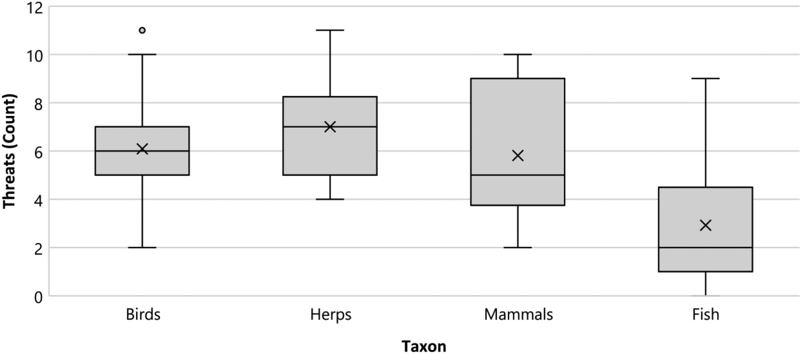
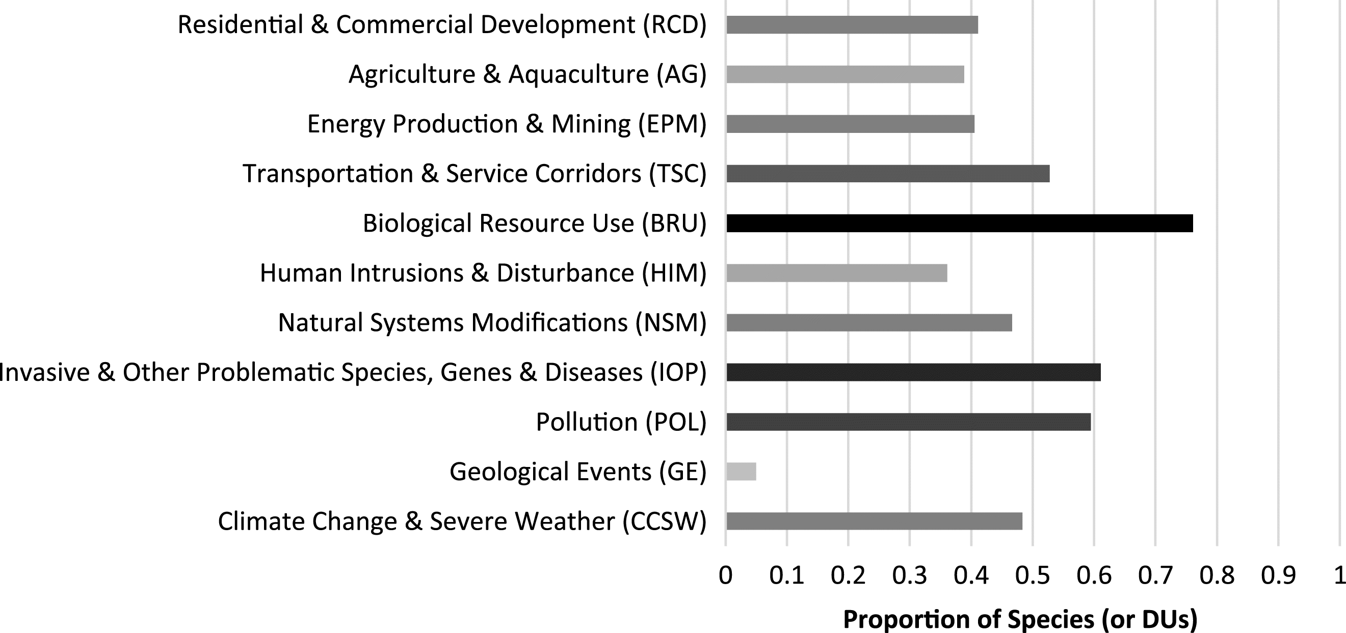
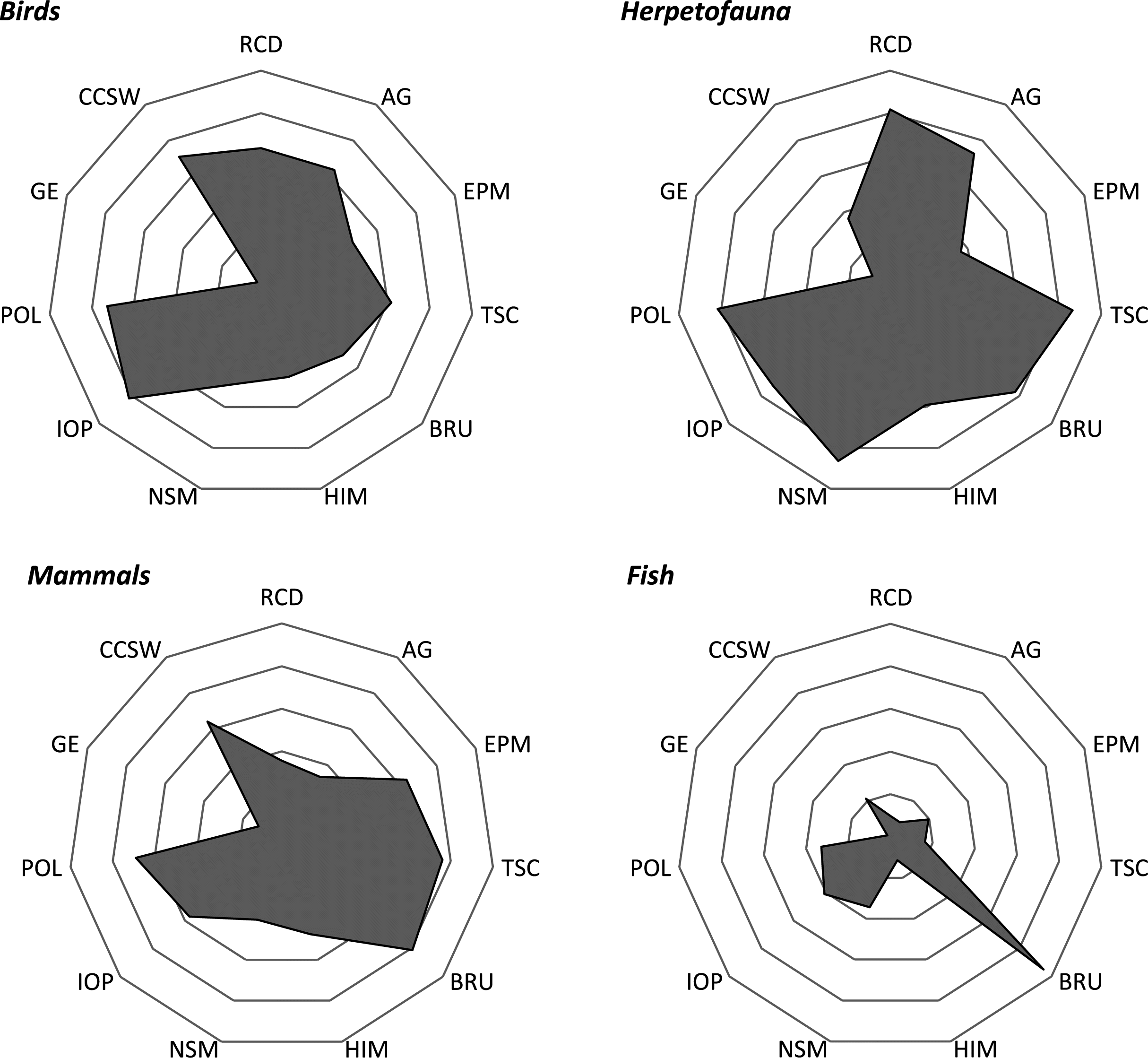
Over three quarters of species had biological resource use (BRU) (76.11%) as a cited threat, which encompasses deliberate and (or) unintentional harvesting effects. Invasive and other problematic species, genes, and diseases (61.11%); pollution (59.44%); and transportation and service corridors (52.78%) were also pervasive, with more than half of species falling into each category. By comparison, the threat of catastrophic geological events was rarely referenced (5.00%) in the analyzed COSEWIC reports (Fig. 1). BRU was the most frequently cited threat among fish species (95.08%) (Fig. 2) and was also frequently mentioned for mammals (80.95%) and herpetofauna (77.27%). Between taxonomic groups, birds and herpetofauna exhibited relatively similar threat distributions (Fig. 2), yet herpetofauna had proportionally more threats cited within their COSEWIC assessments in comparison with other taxa (Fig. 3). The alternative is true for fish, where BRU was frequently the sole threat cited (32.79%), contrasting sharply with the threat profiles of other taxa. In general, however, threats were rarely listed in isolation, as evidenced by a mere 11.11% of species experiencing just one threat. Rather, species were generally affected by multiple threats. The species included in the analysis had 5.06 (±2.77) threats listed on average, with differences among taxonomic groups (Fig. 3).
Fig. 1.
Fig. 1. Proportion of Committee on the Status of Endangered Wildlife in Canada (COSEWIC)-assessed at-risk vertebrate species (or Designatable Units (DU)) exposed to one or more threats in a given International Union for the Conservation of Nature Threat Classification threat category based on information extracted from the most recent COSEWIC status report.
Fig. 2.
Fig. 2. Proportion of taxon-specific species (or Designatable Units) in the sample exposed to one or more threats in a given International Union for the Conservation of Nature Threat Classification threat category based on information extracted from the most recent Committee on the Status of Endangered Wildlife in Canada status report. Threats include residential and commercial development (RCD), agriculture and aquaculture (AG), energy production and mining (EPM), transportation and service corridors (TSC), biological resource use (BRU), human intrusions and disturbance (HIM), natural systems modifications (NSM), invasive and other problematic species, genes, and diseases (IOP), pollution (POL), geological events (GE), and climate change and severe weather (CCSW).
Fig. 3.
Fig. 3. Boxplot representing the number of International Union for the Conservation of Nature Threat Classification threat categories by taxonomic group. X’s represent the average number of threats affecting the species (or Designatable Units) included in this analysis.
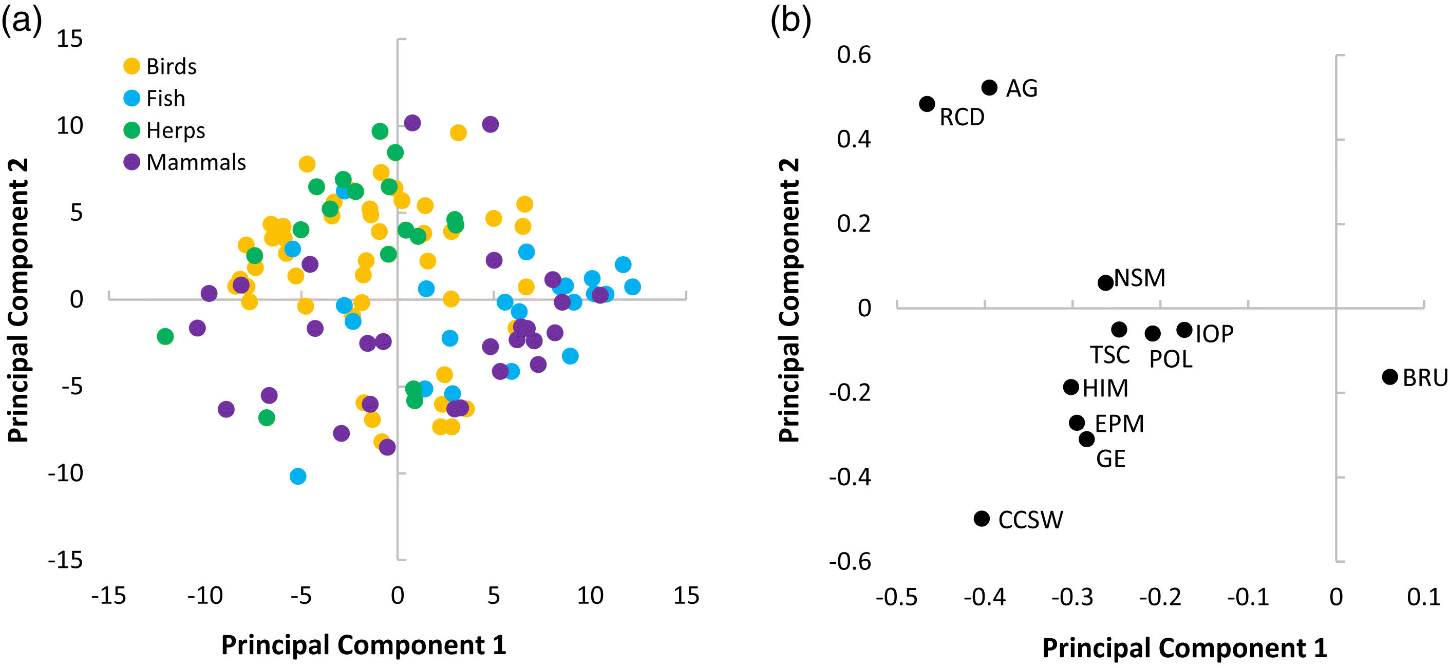
The PCA took 47 iterations for convergence into two PC, with PCs explaining 43.9% of the deviance. Taxonomic patterns among threat profiles were generally apparent (Fig. 4). For instance, mammals occupied similar PCA space, scoring negatively on PC2, while herpetofauna and birds generally scored positively on PC2. Fish were more closely clustered, scoring positively on PC1. Patterns were also evident among threats. BRU was the only threat that scored positively on PC1 correlating to the PCA scores of fish where BRU was the most frequently cited threat and was routinely cited in isolation, representing a highly distinguished threat profile. PCA threats also demonstrated an isolated cluster of residential and commercial development (RCD) and agriculture (AG). Of the 180 COSEWIC-assessed species or DUs comprising four taxonomic groups, 31.67% had a threat profile including both RCD and AG. These were predominantly birds and herpetofauna, which also scored negatively on PC1 and positively on PC2.
Fig. 4.
Fig. 4. (a) Principal component scores for vertebrate species (or Designatable Units) of a particular taxon approximated in a two-dimensional latent space. (b) Corresponding component threats for the 11 International Union for the Conservation of Nature threat classes included in the principal component analysis. Threats include residential and commercial development (RCD), agriculture and aquaculture (AG), energy production and mining (EPM), transportation and service corridors (TSC), biological resource use (BRU), human intrusions and disturbance (HIM), natural systems modifications (NSM), invasive and other problematic species, genes, and diseases (IOP), pollution (POL), geological events (GE), and climate change and severe weather (CCSW).

Analyzing trends in abundance between threats

The top models, selected based on the cumulative sum (≤0.95) of quasi-Akaike weights, encompassed all the explanatory features, suggesting that all variables contributed to the variance explained among the observed proportion of positive years for the time series data (Table 2). The full table of results can be accessed from the Supplementary Material 1 (Table S1).
Table 2.
Table 2. Retained models based on the cumulative sum (≤0.95) of quasi-Akaike weight.
ModelΔQAICWeightMarginal R2Conditional R2TXPAGLPC1PC2PC1 × PC2
TX0.000.170.070.60+
TX + GL0.050.170.080.60+0.34
TX + PC1 × PC21.340.090.100.60+0.01−0.06−0.03
TX + PC1 × PC2 + GL1.970.060.110.60+0.310.00−0.04−0.03
TX + PC11.990.060.070.60+0.01
TX + PA2.020.060.070.60++
TX + PA + GL2.060.060.080.60++0.35
TX + PC1 + GL2.090.060.080.60+0.350.01
GL2.660.050.060.620.73
TX + PC1 × PC2 + PA3.380.030.100.60++0.01−0.06−0.03
TX + PC1 + PC23.770.030.070.60+0.01−0.03
TX + PC1 × PC2 + PA + GL4.000.020.110.60++0.310.00−0.04−0.03
TX + PC1 + PA4.010.020.070.60++0.01
TX + PC1 + PC2 + GL4.120.020.080.60+0.340.00−0.01
PC1 + GL4.640.020.060.620.710.01
RVI0.870.200.460.420.260.21

Note: Weights are ranked in order of performance according to Δquasi-Akaike’s Information Criterion (QAIC; models with ΔQAIC <2 are bolded). Fixed effects include taxon (TX); principal components 1 (PC1) and 2 (PC2); generation length (GL); and data collected predominantly within a protected area (PA). The relative variable importance (RVI) is also included for reference, measured by the sum of the quasi-Akaike weights for models which contain the predictor of interest.

Of the 30 models fit to the data, the top performing model was exclusively comprised of the fixed effect of taxonomic group (TX). Approximately 7.07% of the variation in the proportion of annual increases was explained via the fixed effect of TX (marginal R2), while 59.56% was explained by both the fixed and random effects (conditional R2). Moreover, there were five models where ΔQAIC <2 (bolded in Table 2), all of which contained the fixed effect of TX, and none of which contained protected areas (PA). This highlights the importance of TX in explaining the proportion of annual increases, which is also reflected via its high relative variable importance (RVI) score of 0.87. Conversely, population occurrence (data collection) within PA was a less useful variable in explaining trends in abundance as it was absent from the top five performing models and had a comparatively low RVI of 0.20.
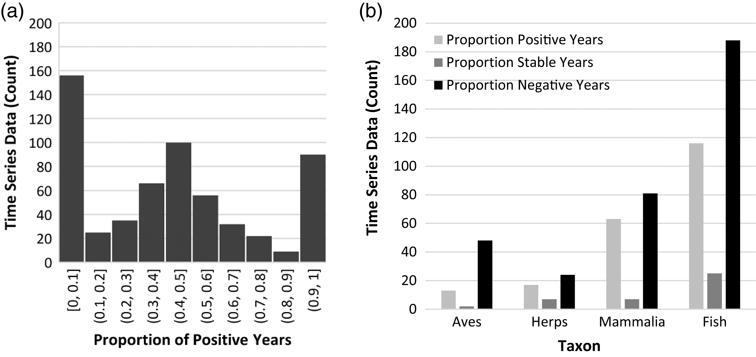
Within the data set, there was a greater proportion of negative years than positive years (Fig. 5)—this is particularly true for at-risk birds that, on average, exhibited more steady trends of decline. There is, however, greater fluctuation in trends over the 1970–2014 time period for fish, herpetofauna, and mammals (Fig. S5). Consequently, the effect of TX on the proportion of annual increases was noteworthy yet differed in the strength of its effect among the four taxonomic classifications.
Fig. 5.
Fig. 5. (a) Histogram of the proportion of positive years for the 591 time series included in the analysis. Values >0.5 would have a greater proportion of positive years within the time series. Alternatively, values <0.5 would have a greater proportion of negative years. (b) The proportion of positive, stable, and negative years within time series, separated by taxonomic group.
Even though the top models (n = 16) encompassed all the explanatory features analyzed, individual comparisons of the null model to models consisting only of individual fixed effects provided insight into the strength of these relationships (Table S3). For instance, the null model was considered a stronger predictor of trends than threat profile (PC1 × PC2) or PAs as determined via comparison to the null. Alternatively, individual models of TX and GL were considerably favored over the null.

Discussion

Representation of data

Birds were the best represented taxonomic group in our analysis, largely attributable to data from the Status of Birds in Canada (ECCC 2015), which aggregates data from bird monitoring surveys across the country including the North American Breeding Bird Survey (Pardieck et al. 2018) and the Christmas Bird Count (NAS 2016). Fish, which represent 43.17% of Canadian at-risk species as designated by COSEWIC, were also well-represented in the analysis as a result of Research Vessel Trawl Survey data from Fisheries and Oceans Canada. These large-scale monitoring programs are valuable in determining large-scale trends, but as shown through the analysis of predictor variables and population trends, they may lack a level of geographic specificity to produce meaningful results.
The low representation of amphibians and reptiles in the data set is consistent with their overall representation in the global LPI database (McRae et al. 2017; Saha et al. 2018). Although the natural history, biology, and physiology of most amphibian and reptile species are generally documented, there is a comparatively poorer understanding of biological population size and distribution—partially attributed to a lack of baseline data and the difficulty in monitoring species of solitary and cryptic behavior (CESCC 2011).

Threat profiles

Given that most species face multiple threats, a determination of (i) which threats are the most prevalent and (ii) which threats act synergistically on population abundance, would seem crucial for the recovery of many species. BRU was the most frequently cited threat to at-risk vertebrate species in our sample, consistent with previous studies, which found BRU as the most frequently cited threat of scientifically assessed at-risk flora and fauna in Canada (Prugh et al. 2010) and worldwide (Maxwell et al. 2016). Importantly, BRU was not merely an effect of the greater number of fish species included in our analysis, given that BRU was among the most frequently cited threats for multiple taxa. In Canada, despite no comparable assessment for 8 years, the similarities of analyses are prevalent: BRU was the most frequently cited threat, followed by invasive and other problematic species, genes and diseases—while catastrophic geological events was last (Prugh et al. 2010).
Conversely, in an analysis of threats extracted from recovery strategies for SARA-listed flora and fauna in Canada, human intrusion and disturbance (recreational, military, and other activities) was the most frequently cited threat (McCune et al. 2013). However, species considered threatened by BRU according to COSEWIC were (i) less likely to be listed under SARA, (ii) infrequently has BRU as a listed threat, and (or) (iii) lacked a final recovery strategy for data extraction (McCune et al. 2013). Consequently, as an example only six marine fish were included in the analysis by McCune et al. (2013) compared to the 41 included in this analysis—all of which had BRU as a listed threat. This bias against listing harvested fish and northern mammals under SARA has been well-documented in the literature (Mooers et al. 2007; Findlay et al. 2009; Creighton and Bennett 2019) and likely contributes to the discrepancies between our analysis and that of McCune et al. (2013).
Within the analysis, threats were rarely listed in isolation. Rather, species were generally affected by multiple, compounding pressures. There were some patterns (e.g., taxonomic groups) where signals could be detected among the distribution of threats. For instance, PCA scores demonstrated an isolated cluster of RCD and AG, likely due to their prevalence in similar geographic space—southern Canada. Given that species richness gradients are strongly correlated to climate, species are concentrated within the southern regions of Canada (Coristine and Kerr 2011) where many at-risk species reach their northern range limits (Gibson et al. 2009). Hotspots of at-risk vertebrates are particularly prevalent in southern Ontario and Quebec, the prairies, and the Okanagan Valley of British Columbia (Coristine and Kerr 2011; WWF Canada 2019)—areas characterized by intensive land-use by agriculture and development (Coristine and Kerr 2011; Coristine et al. 2018). This is particularly true for birds (eBird Canada 2018) and herpetofauna inhabiting the northern periphery of their distribution (Lesbarrères et al. 2014)—taxa that occupy similar PCA space as RCD and AG.
Amphibians and reptiles were considered the most threatened by compounded pressures, with a comparatively greater proportion of threats cited within their respective COSEWIC reports. According to the IUCN Red List, amphibians are the most threatened taxa (Baillie et al. 2010) and often epitomize the current biodiversity crisis (Sodhi et al. 2008). Of the species or DUs assessed by COSEWIC, 65.12% of amphibians and 90.57% of reptiles are designated as at-risk or Extirpated (sararegistry.gc.ca). To put this into perspective, of all flora and fauna assessed by COSEWIC with active designations, 77.33% are designated at-risk or Extirpated, and 19.76% are classified as Not at Risk, underscoring the vulnerability of herpetofauna within national borders. More than any other taxa, herpetofauna are restricted to the southern latitudes of Canada at the northern periphery of their distribution (Lesbarrères et al. 2014), where human footprint is highest (Venter et al. 2016)—which translates into numerous threats for these species.

Analyzing drivers of trends

In general, advancing the understanding of factors—threat profile, TX, GL, and PAs—that influence trends in abundance, may help to prioritize biological attributes, physical elements, and conservation actions to maximize species recovery. Our analysis shows that the biotic factors selected (TX and GL) were considered stronger determinants of population trends in comparison to threat profiles and protected areas. In particular, our results suggest an association between TX and population trends, echoing results of Leung et al. (2017). In the literature, however, there remains mixed evidence of GL as a predictor of population trends or extinction risk (Purvis et al. 2000; Collen et al. 2011). By comparison, PA was not a good predictor of population trends, though a lack of variance may have attributed to the absence of a PA effect—where only 7.95% of population time series had data collection within a PA. Finally, despite the association between taxon and population trends and its apparent correlation with threats as per the PCA results, we found no evidence of the predictive power of threat profiles on the proportion of annual increases for population time series of COSEWIC-assessed at-risk species.
Given that multiple threats are often acting in synergy (Brook et al. 2008), the use of threat profiles was favored over the examination of individual threats, but the approach had limited predictive power and was therefore not as powerful as initially anticipated. Below, we provide a series of justifications as to why, and some insights regarding how these issues could be remedied to strengthen future iterations of this work.

Lack of precise spatial data

PA itself may not be a robust predictor of decline but may improve when paired with regional considerations. For instance, Craigie et al. (2010) found that when considering the individual effect of PA of mammal population trends in Africa, western populations exhibited large declines, eastern populations experienced moderate declines, and southern populations revealed stable or increasing trends. Our analysis did not account for geographical differences due to inadequate spatial data associated with LPI trends. Specifically, population trends were often associated with large regions (e.g., provincial scale), rather than unique or refined geographic locations, limiting our ability to appropriately harness spatial data. Consequently, the absence of an effect of PA may be attributed to variation of population trends within PAs in the absence of regional differences. Nevertheless, PA did not emerge as a statistically significant fixed effect in similar studies (e.g., Spooner et al. 2018) despite the inclusion of spatial data.

Biases and outdated classification of threats

Importantly, the subjective nature of listing threats to species has been well documented for the IUCN Red List (Hayward 2009). The potential bias in listing and further interpretation of these threats can therefore limit quantitative analyses aimed at comparing threat profiles and trends. For example, though nearly half of species in our analysis had Climate Change and Severe Weather (CCSW) as a listed threat, an increased incidence of CCSW categorization was revealed in the analyzed COSEWIC Status Reports. Of the assessed species 62.68% of COSEWIC assessments in the last 5 years had CCSW as a listed threat, compared with 40.62% in the 5 years prior.
In Canada, COSEWIC defines threats as “activities or processes that directly negatively affect the Canadian population” (COSEWIC 2015). In November 2015, COSEWIC approved a threat classification and assessment calculator that applies the IUCN threat classification system. COSEWIC mandated the systematic application of threat classification for all threat categories in future COSEWIC status reports. Under this system, threats are also characterized with respect to “scope”, “severity”, and “timing”, which can be used to generate the relative impact of a given threat. Despite implementation of this detailed and rigorous approach to listing threats, COSEWIC reports conducted prior to 2015, which contributes 90.56% of species in our analysis, were likely prone to greater biases in listing of threats, and interpretation and correlation of listed threats to IUCN categories.

Poor sample size and variation among predictive factors

In our analysis, we were unable to partition out individual taxa owing to poor sample size. Consequently, we struggled to include appropriate cross-taxa measures such as body size, where length is typically recorded for fish and herpetofauna (Froese and Pauly 2016; Santini et al. 2018) and mass is generally used for birds and mammals (Myhrvold et al. 2015). Collen et al. (2011), and we also suggest that a lack of significant predictors could also be attributed to small sample sizes or a lack of variance across given predictors. In our data set, only 7.95% of population time series were within PAs, suggesting that a lack of variance may have attributed to the absence of a PA effect. We were also unable to look at phylogenetically induced effects as fitting genus and species in a nested structure resulted in convergence errors and did not improve model fit.
Recommendations

Prioritization of conservation action

Based on this analysis, it appears that mitigation of BRU would benefit the greatest number of at-risk species in Canada. Critically, mitigation of BRU is more technically, economically, and biologically feasible yielding direct conservation outcomes (Prugh et al. 2010; Hayward 2011; Dirzo et al. 2014), largely via effective legislative and policy changes (Prugh et al. 2010; Hayward 2011). Other threats are comparatively difficult to combat due to their pervasive nature, greater financial cost, need for habitat restoration following abatement of a given threat, and largely indirect biological outcomes (Prugh et al. 2010; Hayward 2011). Importantly, at-risk species threatened by BRU, particularly harvested fish and northern mammals, are frequently denied legal protection under SARA (Mooers et al. 2007; Findlay et al. 2009), epitomizing a lack of political will and bias associated with conservation action in Canada. In addition to SARA, possible tools to combat BRU include the introduction and enforcement of harvest regulations (including bans), regulated sustainable harvest regimes, and establishment of no-take protected areas (Maxwell et al. 2016). While harvest management is frequently proposed, it is rarely sufficiently implemented (Hayward 2011), and many of these tools require strengthening and enhanced application to achieve desired conservation outcomes. In conjunction with harvest regulations, captive breeding and reintroduction of target species (Hayward 2011), and protective eco-labels with strict requirements (i.e., Treves and Jones 2010) can also facilitate wildlife recovery.

Mixed-effects models and methodological improvements

While threat profile was endeavored as a theoretically enhanced approach compared with evaluating singular threats—an association of temporal abundance and threat profile was not unveiled. However, a number of caveats and data limitations exist; therefore, threat profile should not be entirely ignored. Methodological improvements could further yield results that may more appropriately direct conservation action—particularly in the association between trends and threat profiles. Future analyses should focus on data gathering of population trends with precise geographic coordinates, permitting the inclusion of spatial elements (e.g., climate warming and land-use change) as determinants of extinction risk, particularly since a critical determinant of our anthropogenic impact on wildlife encompasses the degree of spatial overlap between human footprint and biodiversity (Tilman et al. 2017). Nevertheless, use of spatial data alone is also ineffective. Canada-wide spatial analyses (Kerr and Cihlar 2004; Kerr and Deguise 2004; Gibbs et al. 2009) have found that urbanization and agricultural areas are correlated with at-risk species or losses of imperiled species. However, though spatial analyses are helpful for informing our human footprint impacts on biodiversity from a geographical perspective, these analyses mask the fact that direct pressures, such as overexploitation, may be threatening wildlife to an equal or greater extent. Ideally, mixed-effect models would include a combination of spatial and categorical components to further analyze the impacts of threats on trends in population abundance. Similarly, incorporation of additional biological and physical factors with sufficient variation may also enhance predictive models and strengthen the possibility of identifying an overall effect. Finally, inclusion of overall threat impact (i.e., scope and severity) may also provide greater accuracy associated with threat profiles as predictors of decline. This approach should reduce bias in the interpretation of threats from COSEWIC reports and enhance data composition for future analyses.

Acknowledgements

We are very grateful to the students and researchers at the University of Ottawa, particularly Sue McKee who provided threat data extracted from COSEWIC reports. We also acknowledge the contributions of the many individuals who have provided data to the Living Planet Index data portal, for public use. We are grateful to Scott Findlay, Robin Freeman, Xavier Harrison, Louise McRae, Emily Giles, and James Snider for providing meaningful feedback and comments on the data set, analysis, and draft manuscript.

References

Baillie JE, Griffiths M, Turvey J, Loh ST, and Collen B. 2010. Evolution lost: status and trends of the world’s vertebrates. Zoological Society of London, London, United Kingdom. 72 p.
Barnes MD, Craigie ID, Harrison LB, Geldmann J, Collen B, Whitmee S, et al. 2016. Wildlife population trends in protected areas predicted by national socio-economic metrics and body size. Nature Communications, 7: 12747.
Barton K. 2016. MuMln: multi-model inference. R package: MuMIn.
Bates D, Maechler M, Bolker B, and Walker S. 2015. Fitting linear mixed-effects models using lme4. R package: lme4.
Bennett P, and Owens IPF. 1997. Variation in extinction risk among birds: chance or evolutionary predisposition. Proceedings of the Royal Society B, 264: 401–408.
Brook BW, Sodhi NS, and Bradshaw JA. 2008. Synergies among extinction drivers under global change. Trends in Ecology and Evolution, 23(8): 453–460.
Canadian Council on Ecological Areas (CCEA). 2017. Conservation Areas Reporting and Tracking System (CARTS), with Quebec data used by permission (data are current as of 2017) [online]: Available from http://www.ccea.org/download-carts-data/.
Canadian Endangered Species Conservation Council (CESCC). 2011. Wild Species 2010: The General Status of Species in Canada. National General Status Working Group, Ottawa, Ontario. 302 p.
Cardillo M, Mace GM, Jones KE, Bielby J, Bininda-Emonds ORP, Sechrest W, et al. 2005. Multiple causes of high extinction risk in large mammal species. Science, 309(5738): 1239–1241.
Collen B, Loh J, Whitmee S, McRae L, Amin R, and Baillie JEM. 2009. Monitoring change in vertebrate abundance: the Living Planet Index. Conservation Biology, 23(2): 317–327.
Collen B, McRae L, Deinet S, De Palma A, Carranza T, Cooper N, et al. 2011. Predicting how populations decline to extinction. Philosophical Transactions of the Royal Society B, Biological Sciences, 366: 2577–2586.
Committee on the Status of Endangered Wildlife in Canada (COSEWIC). 2015. Instructions for preparing COSEWIC status reports [online]: Available from https://www.canada.ca/en/environment-climate-change/services/committee-status-endangered-wildlife/instructions-preparing-status-reports.html.
Committee on the Status of Endangered Wildlife in Canada (COSEWIC). 2016. COSEWIC definitions and abbreviations [online]: Available from https://www.canada.ca/en/environment-climate-change/services/committee-status-endangered-wildlife/definitions-abbreviations.html.
Coristine LE, and Kerr JT. 2011. Habitat loss, climate change, and emerging conservation challenges in Canada. Canadian Journal of Zoology, 89: 435–451.
Coristine LE, Jacob AL, Schuster R, Otto SP, Baron NE, Bennett NJ, et al. 2018. Informing Canada’s commitment to biodiversity conservation: a sciences-based framework to help guide protected areas designation through Target 1 and beyond. Facets, 3: 531–562.
Craigie ID, Baillie JEM, Balmford A, Carbone C, Collen B, Green RE, et al. 2010. Large mammal population declines in Africa’s protected areas. Biological Conservation, 143: 2221–2228.
Creighton MJA, and Bennett JR. 2019. Taxonomic biases persist from listing to management for Canadian species at risk. Écoscience, 26(4): 315–321.
Daskalova GN, Myers-Smith IH, and Godlee JL. 2018. Rarity and conservation status do not predict vertebrate population trends. bioRxiv, 27898.
Davidson AD, Hamilton MJ, Boyer AG, Brown JH, and Ceballos G. 2009. Multiple ecological pathways to extinction in mammals. Proceedings of the National Academy of Sciences of the United States of America, 106(26): 10702–10705.
Dirzo R, Young HS, Galetti M, Ceballos G, Isaac NJB, and Collen B. 2014. Defaunation in the Anthropocene. Science, 345(6195): 410–406.
eBird Canada. 2018. Hotspot interactive map [online]: Available from https://ebird.org/canada/hotspots.
Environment and Climate Change Canada (ECCC). 2015. Status of birds in Canada 2014. Canadian Wildlife Service, Environment Canada, Gatineau, Quebec. Data contributed in 2016.
Erhlén J, and Morris WF. 2015. Predicting changes in the distribution and abundance of species under environmental change. Ecology Letters, 18: 303–314.
Findlay CS, and McKee S. 2018. Canadian species at risk database. University of Ottawa, Ottawa, Ontario.
Findlay CS, Elgie S, Giles B, and Burr L. 2009. Species listing under Canada’s Species at Risk Act. Conservation Biology, 23(6): 1609–1617.
Freeman R, McRae L, Deinet S, Amin R, and Collen B. 2017. rlpi: tools for calculating indices using the Living Planet Index method. R package.
Froese R, and Pauly D. 2016. FishBase [online]: Available from www.fishbase.org.
Gibbs KE, Mackey RL, and Currie DJ. 2009. Human land use, agriculture, pesticides and losses of imperiled species. Diversity and Distributions, 15: 242–253.
Gibson SY, Van der Marel RC, Starzomski BM. 2009. Climate change and conservation of leading-edge peripheral populations. Conservation Biology, 23(6): 1369–1373.
Hardesty-Moore M, Deinet S, Freeman R, Titcomb GC, Dillon EM, Stears K, et al. 2018. Migration in the Anthropocene: how collective navigation, environmental systems and taxonomy shape the vulnerability of migratory species. Philosophical Transactions of the Royal Society B, Biological Sciences, 373(1746).
Harrison XA, Donaldson L, Correa-Cano ME, Evans J, Fisher DN, Goodwin CED, et al. 2018. A brief introduction to mixed effects modelling and multi-model inference in ecology. PeerJ, 6: e4794.
Hayward MW. 2009. The need to rationalize and prioritize threatening processes used to determine threat status in the IUCN Red List. Conservation Biology, 23(6): 1568–1576.
Hayward MW. 2011. Using the IUCN Red List to determine effective conservation strategies. Biodiversity and Conservation, 20(12): 2563–2573.
Hoffmann M, Hilton-Taylor C, Angulo A, Böhm M, Brooks TM, Butchart SHM, et al. 2010. The impact of conservation on the status of the world’s vertebrates. Science, 330(6010): 1503–1509.
Kerr JT, and Cihlar J. 2004. Patterns and causes of species endangerment in Canada. Ecological Applications, 743–753.
Kerr JT, and Deguise I. 2004. Habitat loss and the limits to endangered species recovery. Ecology Letters, 7: 1163–1169.
Korner-Nievergelt F, Roth T, von Felten S, Guelat J, Almasi B, and Korner-Nievergelt P. 2015. Bayesian data analysis in ecology using linear models with R. R package: blmeco.
Landgraf AJ, and Lee Y. 2015. Dimensionality reduction for binary data through the projection of natural parameters: Technical Report 890. Ohio State University, Columbus, Ohio. arXiv:1510.06112v1.
Lawler JJ, Campbell SP, Guerry AD, Kolozsvary MB, O’Connor RJ, and Seward LCN. 2002. The scope and treatment of threats in endangered species recovery plans. Ecological Applications, 12(3): 663–667.
Lesbarrères D, Ashpole SL, Bishop CA, Bloiun-Demers G, Brooks RJ, Echaubard P, et al. 2014. Conservation of herpetofauna in northern landscapes: threats and challenges from a Canadian perspective. Biological Conservation, 170: 48–55.
Leung B, Greenberg DA, and Green DM. 2017. Trends in mean growth and stability in temperate vertebrate populations. Diversity and Distributions, 00: 1–9.
Loh J, Green RE, Ricketts T, Lamoreux J, Jenkins M, Kapos V, and Randers J. 2005. The Living Planet Index: using species population time series to track trends in biodiversity. Philopsophical Transactions of the Royal Society B, Biological Sciences, 260: 289–295.
Marconi V, McRae L, Muller H, Currie J, Whitmee S, Gadallah F, and Freeman R. Coverage of a national biodiversity indicator: data of different quality show diverging trends (in preparation).
Maxwell SL, Fuller RA, Brooks TM, and Watson JEM. 2016. Biodiversity: the ravages of guns, nets and bulldozers. Nature, 536: 143–145.
McCune JL, Harrower WL, Avery-Gomm S, Brogan JM, Csergö AM, Davidson LNK, et al. 2013. Threats to Canadian species at risk: an analysis of finalized recovery strategies. Biological Conservation, 166: 254–265.
McRae L, Deinet S, and Freeman R. 2017. The diversity-weighted Living Planet Idex: Controlling for taxonomic bias in a global biodiversity indicator. PLoS ONE, 12(1): e0169156.
Mooers AØ, Prugh LR, Festa-Bianchet M, and Hutchings JA. 2007. Biases in legal listing under Canadian Endangered species legislation. Conservation Biology, 21(3): 572–575.
Myhrvold NP, Baldridge E, Chan B, Sivam D, Freeman DL, and Ernest SKM. 2015. An amniote life history database to perform comparative analyses with birds, mammals, and reptiles. Ecology, 96(11): 3109.
National Audubon Society (NAS). 2016. The Christmas bird count historical results [online]: Available from http://www.christmasbirdcount.org.
Pardieck KL, Ziolkowski DJ Jr, Lutmerding M, and Hudson MAR. 2018. North American breeding bird survey dataset 1966-2017, version 2017.0. US Geological Survey, Patuxent Wildlife Research Center, Laurel, Maryland.
Prugh LR, Sinclair ARE, Hodges KE, Jacob AL, and Wilcove DS. 2010. Reducing threats to species: threat reversibility and links to industry. Conservation Letters, 3: 267–276.
Purvis A, Gittleman JL, Cowlishaw G, and Mace GM. 2000. Predicting extinction risk in declining species. Proceedings of the Royal Society B, 267: 1947–1952.
R Core Team. 2017. R: a language and environment for statistical computing. R Foundation for Statistical Computing, Vienna, Austria.
Saha A, McRae L, Dodd CK Jr, Gadsden H, Hare KM, Lukoschek V, et al. 2018. Tracking global population trends: population time-series data and a Living Planet Index for reptiles. Journal of Herpetology, 52(3): 259–268.
Salafsky N, Salzer D, Stattersfield AJ, Hilton-Taylor C, Neugarten R, Butchart SHM, et al. 2008. A standard lexicon for biodiversity conservation: unified classifications of threats and actions. Conservation Biology, 22(4): 897–911.
Santini L, Benítez-López A, Ficetola GF, and Huijbregts MAJ. 2018. Length-mass allometries in amphibians. Integrative Zoology, 13: 36–45.
Sodhi NS, Bickford D, Diesmos AC, Lee TM, Koh LP, Brook BW, et al. 2008. Measuring the meltdown: drivers of global amphibian extinction and decline. PLoS ONE, 3(2): e1636.
Spooner FEB, Pearson RG, and Freeman R. 2018. Rapid warming is associated with population decline among terrestrial birds and mammals globally. Global Change Biology, 24: 4521–4531.
Tilman D, Clark M, Williams DR, Kimmel K, Polasky S, and Packer C. 2017. Future threats to biodiversity and pathways to their prevention. Nature, 546: 73–81.
Treves A, and Jones SM. 2010. Strategic tradeoffs for wildlife-friendly eco-labels. Frontiers in Ecology and the Environment, 8(9): 491–498.
Venter O, Sanderson EW, Magrach A, Allan JR, Beher J, Jones KR, et al. 2016. Sixteen years of change in the global terrestrial human footprint and implications for biodiversity conservation. Nature Communications, 7: 12558.
World Wildlife Fund Canada (WWF Canada). 2017. Living Planet Report Canada: a national look at wildlife loss. World Wildlife Fund, Toronto, Ontario.
World Wildlife Fund Canada (WWF Canada). 2019. Wildlife Protection Assessment: a national habitat crisis. World Wildlife Fund, Toronto, Ontario.

Supplementary material

Supplementary Material 1 (DOCX / 280 KB)
Supplementary Material 2 (XLSX / 87 KB)

Information & Authors

Information

Published In

cover image FACETS
FACETS
Volume 5Number 1January 2020
Pages: 49 - 66
Editor: Jeremy Kerr

History

Received: 22 March 2019
Accepted: 4 December 2019
Version of record online: 3 February 2020

Data Availability Statement

All relevant data are within the paper and Supplementary Material.

Key Words

  1. biodiversity loss
  2. Living Planet Index
  3. wildlife threats
  4. COSEWIC

Sections

Subjects

Plain Language Summary

The combination of threats at-risk species face does not necessarily predict trends in population abundance

Authors

Affiliations

Jessica Currie [email protected]
World Wildlife Fund Canada, 410 Adelaide Street West, Toronto, ON M5V 1S8, Canada
Valentina Marconi
Institute of Zoology, Zoological Society of London, Regent’s Park, London NW1 4RY1S8, UK

Author Contributions

JC conceived and designed the study.
JC performed the experiments/collected the data.
All analyzed and interpreted the data.
All contributed resources.
All drafted or revised the manuscript.

Competing Interests

The authors have declared that no competing interests exist.

Metrics & Citations

Metrics

Other Metrics

Citations

Cite As

Export Citations

If you have the appropriate software installed, you can download article citation data to the citation manager of your choice. Simply select your manager software from the list below and click Download.

Cited by

1. Past, present, and future of the Living Planet Index
2. Multiple impacts of invasive species on species at risk: a case study in British Columbia, Canada
3. CAN-SAR: A database of Canadian species at risk information
4. Threats to Neglected Biodiversity: Conservation Success Requires More Than Charisma
5. Assessing the representation of species included within the Canadian Living Planet Index
6. Population declines among Canadian vertebrates: But data of different quality show diverging trends
7. The biodiversity crisis in Canada: failures and challenges of federal and sub-national strategic and legal frameworks

View Options

View options

PDF

View PDF

Get Access

Media

Media

Other

Tables

Share Options

Share

Share the article link

Share on social media