Open access

Population structure of lake whitefish (Coregonus clupeaformis) from the Mississippian lineage in North America

Publication: FACETS
9 June 2022

Abstract

The lake whitefish (Coregonus clupeaformis) is a commercially valuable freshwater species with a broad distribution in North America. Some phylogeographic work has been done on this species, but little is known about genetic population subdivision among populations of the widely dispersed Mississippian lineage. We used 3,173 single nucleotide polymorphisms in 508 lake whitefish from 22 different lakes to examine population structure across central Canada and the United States. Bayesian clustering, ordination, and fixation indices identified population subdivision that largely reflected geographic distance and hydrological connectivity, with greater differentiation between lakes that are farther apart. Population subdivision was hierarchical, with greater differentiation between Canadian provinces and less differentiation based on river basins within provincial boundaries. Interestingly, isolation by distance alone was not sufficient to account for all of the observed genetic differentiation among populations. We conclude that important components of lake whitefish genetic diversity are present at different spatial scales, and that populations within the Mississippian lineage have differentiated widely across their range.

Introduction

The lake whitefish (Coregonus clupeaformis) is an important species economically, ecologically, and culturally throughout northern North America. In Canada, this cold-water species is found from Yukon to Labrador and makes up the second largest freshwater fishery by landings (Lindsey and Woods 1970; Scott and Crossman 1973; Bernatchez and Dodson 1990; Mee et al. 2015; DFO 2016; Isermann et al. 2020). In the Great Lakes, lake whitefish represent the largest and oldest commercial fishery, with their near shore spawning enabling high catch rates using gill-nets (Kinnunen 2003; Eberner et al. 2008; Rennie et al. 2009). Lake whitefish also serve as an important energy conduit from benthic to pelagic sources, and function to couple nearshore and offshore habitats (Nalepa et al. 2005; Rennie et al. 2009; Eberner et al. 2010). Further, they are an important component of Indigenous culture through subsistence fisheries (Eberner et al. 2008). The lake whitefish is facing serious pressures across its range through over-fishing, invasive species, and habitat and environmental changes, which have already resulted in declines in body condition and growth, commercial yields, and extirpation in some areas (Brenden et al. 2010; Bence et al. 2019; Renik et al. 2020). Even though the lake whitefish is one of the most valuable fisheries across its range, very little is known about genetic population subdivision and diversity outside of the Great Lakes.
Effective management of lake whitefish in North America will benefit from an improved understanding of the evolutionary history and genetic differentiation of the species on multiple spatial scales. During the Pleistocene glaciation the extreme climate created geographically and temporally isolated refugia for fish populations (Mee et al. 2015). Glaciation resulted in four distinct phylogenetic lineages of lake whitefish across North America, the Beringian, Nahanni, Mississippian, and Atlantic, which have been identified using mitochondrial DNA (mtDNA; Bernatchez and Dodson 1991; Foote et al. 1992; Mee et al. 2015). The largest refugium was created by the ice-free portions of the Mississippi river drainage, the Mississippian refugium, and fish from this lineage colonized over 5 million km2 from Alberta to Quebec when the glaciers receded (Mee et al. 2015). MtDNA analysis provides broadscale lineage data, but it only represents a small portion of the evolutionary history and genetic differentiation within a species (Liu et al. 2012). Neutral population subdivision has been examined using traditional markers within small regions, especially within the Great Lakes (Franzin and Clayton 1977; Casselman et al. 1981; Bernatchez and Dodson 1991; Foote et al. 1992; VanDeHey et al. 2009; Stott et al. 2010, 2011; Mee et al. 2015). However, very little population genetic work has been done on lake whitefish within the largest post-glacial lineage group, and never on a broad geographic scale.
The integration of genomics with morphological, biological, and physiological traits enables the identification of distinct populations and has vastly improved stock identification and assessment (Wenne et al. 2007; Allendorf et al. 2010; Isermann et al. 2020; Lu and Luo 2020; Papa et al. 2020). The preservation of local populations is vital to ensure the maintenance of genetic diversity within a species (Wenne et al. 2007; Nielsen et al. 2009; Reitzel et al. 2013; Flanagan et al. 2018). The identification of local genetic groups is improved by incorporating regions of the genome influenced by local adaptation, as neutral structure does not provide the full relationship between groups of individuals (Allendorf et al. 2010; Hemmer-Hansen et al. 2014; Ovenden et al. 2015; Valenzuela-Quinonez 2016; Vu et al. 2020). High throughput sequencing enables large-scale genomic analyses of single nucleotide polymorphisms (SNPs) throughout the genome with different evolutionary histories (Davey et al. 2011). These advances can help to provide better insight into the genetic diversity of local populations and help to prioritize management of stocks on multiple scales.
Here we present the largest broadscale population genomic study yet conducted on lake whitefish across the central portion of their North American range. We used nextRAD sequencing of thousands of SNPs to examine levels of genetic diversity and differentiation among lake whitefish populations over a broad geographic scale within the Mississippian refugium. We hypothesized that on a broadscale, lake whitefish populations would be subdivided based on hydrological connectivity and geographic distance. This study provides novel insights into fundamental aspects of population subdivision and the distribution of genetic diversity in lake whitefish and provides a useful baseline for understanding relevant scales for management and conservation.

Materials and methods

Sample collection, DNA isolation, and sequencing

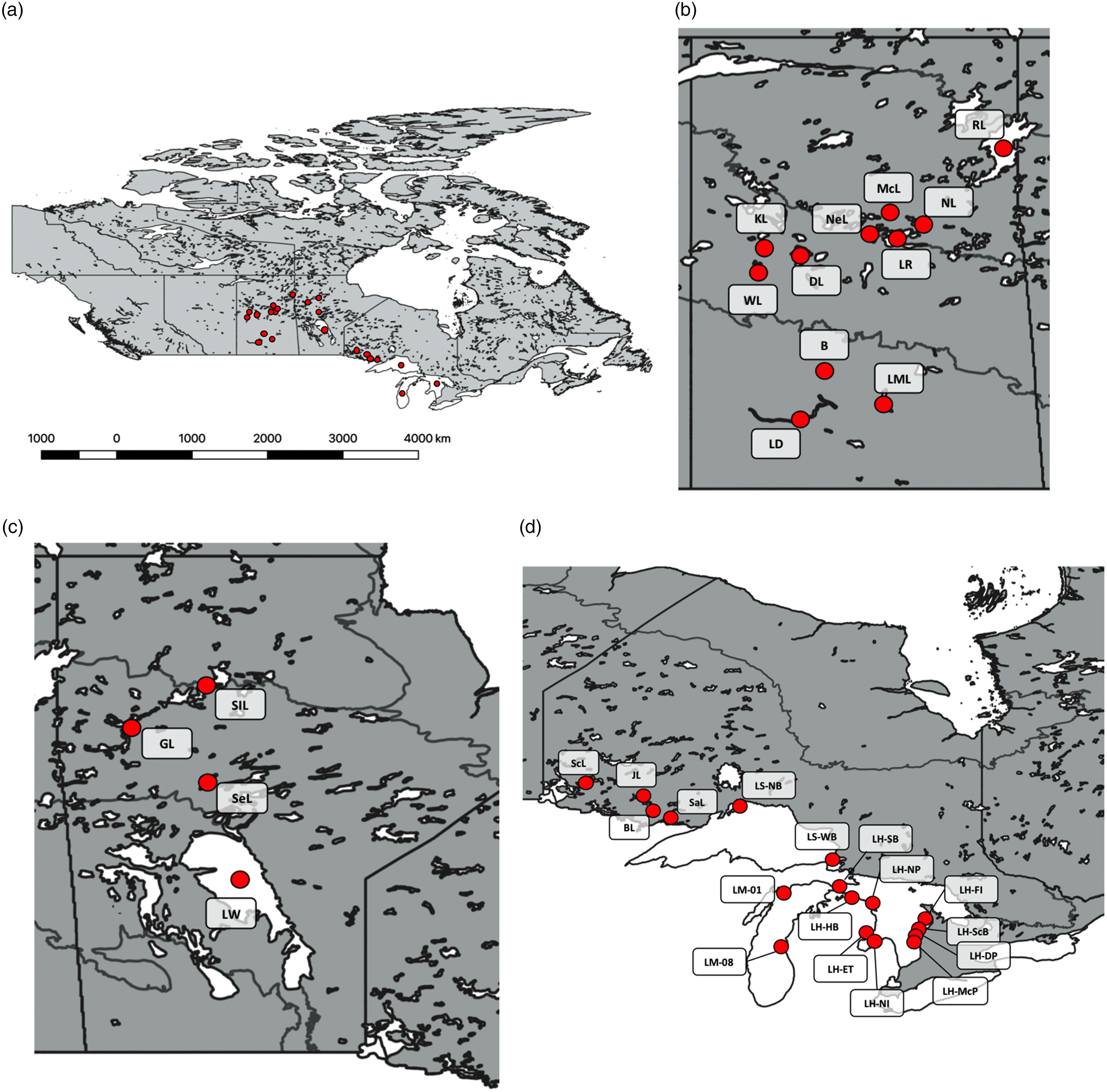
Adult lake whitefish were collected from 22 lakes across central Canada from Saskatchewan to Ontario, and from several sites in the United States from Lakes Michigan and Huron (Table 1; Fig. 1). These lakes were opportunistically sampled to encompass substantial environmental variance in different ecozones and drainages based on location and lake characteristics and to encompass a large geographic area occupied by fish derived from a single glacial refugium (Mississipian; Fig. 1; Table 1; Supplementary Material 2, Table S1). Lake whitefish sampled from multiple sites within a lake were treated as an aggregate in our analyses. Fish were primarily collected through government agencies, commercial fishermen, and fish processing plants. Either dorsal muscle tissue or a fin clip was collected and stored in lysis buffer (4.0M urea/0.2M NaCl/0.1M Tris–HCl, pH 8.0/0.5% n-laurylsarcosine/0.1 M 1,2-cyclo-hexanediamine) for genetic analyses (Table 1). All animal research was approved by the University of Regina President’s Committee on Animal Care, following the guidelines of the Canadian Council on Animal Care. The approved Animal Use Protocol was AUP 11–13 “Population and Conservation Genetics of Freshwater Fish”.
Table 1.
Table 1. Collection data for 508 lake whitefish (Coregonus clupeaformis) samples from 22 lakes across central Canada and the United States.
LakeSiteLatitudeLongitudeDrainageSub-drainageYearTotal (N)Tissue
Great Lakes
Lake HuronLH-ET43.906−83.672Atlantic OceanGreat Lakes201214Muscle
 LH-NI43.878−83.435  201214Muscle
 LH-NP45.395−83.486  201214Muscle
 LH-HB45.502−84.033  201214Muscle
 LH-SB45.981−84.497  201215Muscle
 LH-ScB44.355−81.617  201217Muscle
 LH-DP41.298−81.609  20129Muscle
 LH-MP44.258−81.617  201217Muscle
 LH-FI44.709−80.312  201214Muscle
Lake MichiganLM-0143.131−86.414Atlantic OceanGreat Lakes201220Pectoral fin
 LM-0845.628−86.848  201220Pectoral fin
Lake SuperiorLS-WB46.773−84.607Atlantic OceanGreat Lakes201619Pectoral fin
 LS-NB48.869−87.901  201619Pectoral fin
Winnipeg/Nelson
Burt LakeBL48.295−91.556Hudson BayLake Winnipeg20168Pectoral fin
Jean LakeJL48.53−91.753Hudson BayLake Winnipeg201618Pectoral fin
Saganaga LakeSaL48.25−90.923Hudson BayLake Winnipeg201619Pectoral fin
Schistose LakeScL49.155−93.061Hudson BayLake Winnipeg201614Pectoral fin
Lake WinnipegLW53.319−97.938Hudson BayNelson River201620Pectoral fin
Setting LakeSeL55.065−98.589Hudson BayNelson River201617Pectoral fin
Churchill
South Indian LakeSIL57.055−98.618Hudson BayChurchill River201620Pectoral fin
Granville LakeGL56.254−100.6Hudson BayChurchill River201620Pectoral fin
Reindeer LakeRL57.564−102.143Hudson BayChurchill River201620Pectoral fin
Mackay LakeMcL55.458−104.931Hudson BayChurchill River201216Muscle
Nemieben LakeNeL55.271−105.503Hudson BayChurchill River2009/1010Muscle
Nunn LakeNL55.234−104.316Hudson BayChurchill River201120Muscle
Lac La RongeLR55.174−104.448Hudson BayChurchill River201020Pectoral fin
Keeley LakeKL54.913−108.113Hudson BayChurchill River20116Muscle
Dore LakeDL54.756−107.272Hudson BayChurchill River201520Muscle
Waterhen LakeWL54.491−108.433Hudson BayChurchill River201113Muscle
South Saskatchewan/Qu’appelle
Blackstrap LakeB51.786−106.439Hudson BaySouth Saskatchewan River201519Muscle
Lake DiefenbakerLD51.098−106.638Hudson BaySouth Saskatchewan River201516Adipose fin
Last Mountain LakeLML50.84−105.072Hudson BayQu’appelle River20106Muscle

Note: Sample sites in Lake Huron are East Tawas (ET), North Island (NI), North Point (NP), Hammond Bay (HB), Search Bay (SB), Scougall Bay (ScB), Douglas Point (DP), McRae Point (MP) and Fishing Islands (FI) and in Lake Superior are Whitefish Bay (WB) and Nipigon Bay (NB).

Fig. 1.
Fig. 1. Map of the lakes sampled (a) across central Canada, (b) in Saskatchewan, (c) in Manitoba, and (d) in Ontario. Site abbreviations can be found in Table 1. Lines within provinces represent different ecozones. The base map shape file is from the Atlas of Canada, provincial boundaries shape file is from GADM and the ecozone shape file is from the Government of Canada.
DNA was extracted from 20 mg of tissue following the manufacturers guidelines (Genomic DNA Isolation Kit, Norgen Biotech Corp., Ontario, Canada), except for extending the proteinase K digestion to 8-12 hours and the addition of 28 U of RNAse A (Qiagen Inc., Ontario, Canada). Following isolation, DNA was quantified using a Qubit 2.0 Fluorometer (Life Technologies Inc., Ontario, Canada), and the quality was assessed using a 1% agarose gel (E-Gel; Thermo Fisher Scientific, Canada).
Samples were prepared using an amplification-based reduced representation library preparation approach to accommodate varying levels of DNA quality and low amounts of input DNA. To generate the sequencing library, genomic DNA was converted into Nextera-tagmented reductively amplified DNA sequencing (nextRAD) genotyping-by-sequencing libraries (SNPsaurus, Oregon, USA), as described by Russello et al. (2015). Briefly, genomic DNA was first digested with the Nextera reagent (Illumina, Inc., British Columbia, Canada), which randomly fragments the genome using a transposase. The Nextera reagent also ligates short adapter sequences to the ends of the fragments. For high-quality (mostly intact, high molecular weight DNA) samples the Nextera reaction included 20 ng of input DNA; for moderately degraded (sheared; fragments < 5 Kb) samples we used 40 – 60 ng of input DNA to compensate for degradation (Supplementary Material 1). Fragmented DNA was then amplified with a primer matching the adaptor sequence and extending 10 nucleotides into the genomic DNA with the selective sequence 5′-GTGTAGAGCC-3′. Following hybridization of the primers, PCR amplification was done with an annealing temperature of 72 °C for 27 cycles. This allowed for selective hybridization and amplification of fragments that paired with the primer sequence, as well as the incorporation of individual barcodes. We generated nextRAD sequencing data from two independent libraries and sequencing runs (Illumina HiSeq 2500 with 150 bp single end reads; University of Oregon): (i) Lake Huron and (ii) the rest of the lakes in the study. The data from the first run were used in an extensive examination of the influence of bioinformatics parameters on population differentiation by Graham et al. (2020). The second nextRAD dataset was generated from two different lanes on the sequencer; we used data from both sets for the analyses presented here.

Data quality filtering and genotyping parameters

Raw sequence files were first processed using TRIMMOMATIC (Bolger et al. 2014) to remove Nextera adaptors. Reads were then visualized using FASTQC (Andrews 2010) to ensure the removal of Nextera adaptors and examine read quality. All sequences were then analyzed using STACKS version 1.48 (Catchen et al. 2013; Rochette and Catchen 2017). The process_radtags script was used to remove any reads with uncalled bases, discard reads with an average quality score below Q10 or that failed the Illumina chastity filter, and truncate the reads to 150 base pairs. The optimal distance allowed between stacks (-M in ustacks), the minimum sequencing depth (-m in ustacks) and the number of mismatches allowed between sample loci (-n in cstacks) were optimized using the r80 rule as recommended by Paris et al. (2017), and optimized parameters were determined to be M = 3, m = 3, and n = 3. The ustacks script was run using a minimum sequencing depth of 3 (-m), a maximum distance of 3 base pairs allowed between stacks (-M), and a maximum distance of 3 base pairs allowed to align secondary reads (-N). The removal algorithm was also enabled to remove highly repetitive stacks. Following ustacks, a catalog of consensus loci was generated using the cstacks script with at least 5 individuals from each lake with reads near the mean of all samples. More individuals were included from lakes with multiple sample locations (Table 1). This was done to reduce the complexity of the catalog while still capturing the genetic diversity within each lake. The catalog was assembled with a mismatch value of 3 between samples (-n) as determined above. Following generation of the catalog, individual stacks were searched against the catalog using the sstacks script. Finally, the populations script was run to export SNPs. To avoid bias in downstream population structuring as shown by Graham et al. (2020), a population map with no specified populations was used to export data. We analyzed only the first SNP in each locus, and loci had to be present in at least 70% of individuals to be included in the final dataset. Requiring loci to be present in 70% of individuals is an effective means of focusing analyses on loci that are widely represented across the entire sampling region and reduces the influences of missing data (O’Leary et al. 2018; Larson et al. 2020). Minimum minor allele frequency was 0.05.
The influence of missing data on the final dataset was examined using the missing_visualization() function in the grur package in R (Gosselin 2018; R Core Team 2020). A principal coordinate analysis was run to create an isolation by missingness (IBM) plot based on the presence/absence of genotypes within individuals across sample sites. Further, individuals with more than 70% missing data were removed from subsequent analyses. Following the analysis of missing data, loci were checked for conformation to Hardy–Weinberg Equilibrium (HWE; P < 0.01). HWE analysis was done using the filter_hwe() function in the radiator package, which uses the same function as implemented in PLINK 1.07 (Purcell et al. 2007). Loci that did not conform to HWE in 11 or more of the 22 sampled sites were used to create an exclusion list for analyses requiring HWE as an underlying assumption.

Population differentiation analyses

Following quality control, descriptive statistics were calculated for each population. The nucleotide diversity (π) was calculated using the pi() function in radiator. Observed heterozygosity (HO), expected heterozygosity within populations assuming HWE (HS), and the inbreeding coefficient (GIS) were calculated in GENODIVE (Meirmans 2020). The expected heterozygosity (HS) within subpopulations is also known as the gene diversity and includes corrections for sampling bias (Nei 1987). Population diversity and differentiation metrics were calculated based on lake and sub-drainage.
Isolation-by-distance (IBD) was tested using a mantel test in the ade4 R package with 999 replicates (Dray and Dufour 2007). The genetic distance matrix was created using Edwards’ distance to reflect the distance between populations based on gene frequencies in the adegenet package. The geographical distance matrix was generated using the Universal Transverse Mercator coordinate system. As the IBD analysis is statistically flawed (Meirmans 2020), distance-based Moran eigenvector maps (dbMEMs) were also used to determine if spatial factors are important for partitioning genetic variance. This analysis is used to control for signals generated by neutral processes, such as those produced from population structure through IBD (Excoffier et al. 2009; Forester et al. 2018; Xuerub et al. 2018). The Euclidean distances between sample sites were used to compute dbMEMs to decompose the relationships into spatial variables (Dray et al. 2006; Xuerub et al. 2018). The adespatial package was used in R to compute the dbMEMs (Dray et al. 2021). Significant dbMEMs were determined using a forward selection procedure (Blanchet et al. 2008).
Three different population structure analyses were performed on the final SNP dataset using: (i) pairwise fixation indices (FST), (ii) maximum likelihood cluster analysis, and (iii) ordination. As a result of assumptions underlying the analyses, only the loci in HWE were used for both the FST and maximum likelihood analyses, while all loci were used in the ordination approach. The FST analysis was conducted by first computing a distance matrix for all sites using an analysis of molecular variance (AMOVA; Excoffier et al. 1992), and GENODIVE was then used to compute pairwise FST between sample sites using 5,000 permutations (Meirmans 2020). The maximum likelihood analysis was performed using the program ADMIXTURE to estimate the ancestry coefficient of each individual using a maximum likelihood approach (Alexander et al. 2009; Zhou et al. 2011). The cross-validation approach was used in ADMIXTURE to determine the number of populations (K) with the best predictive accuracy (Alexander et al. 2009; Zhou et al. 2011). Following the maximum likelihood analysis, the R package pophelper was used to visualize the output (Francis 2016). The ordination analysis was conducted using discriminant analysis of principal components (DAPC) in the adegenet program using the original population groupings (Jombart 2008; Jombart and Ahmed 2011). The DAPC plot was generated in each analysis using the optim_a_score() function to determine the optimal number of principal components to avoid over-fitting the data.

Results

Data quality filtering and genotyping parameters

Following the removal of the Nextera adapters there was a total of 1,911,624,117 reads with an average of 3,740,947 (SD = 2,191,292) reads per individual. After cleaning and trimming in process_radtags there were 3,242,831 (SD = 1,984,622) average reads per individual. The STACKS modules were run to generate a catalog with 3,221,783 markers. This catalog was generated using 124 individuals, each with average numbers of reads. Following sstacks, there was an average of 77,339 (SD = 37,161) matched loci per individual. Filtering and export in the populations module resulted in a total of 3,173 polymorphic SNP loci identified within the dataset.
Following inspection for missing data using grur, 27 individuals with less than 30% of variable sites genotyped were removed from the analysis, resulting in 481 individuals. Overall, the average percentage of missing data was 18.9% (SD = 14.1%). The IBM plot generated showed that there was no evidence of major biases or clustering of sites based on patterns of missingness for PCo1, explaining 27% of the variance (Supplementary Material 2, Fig. S1). Some individuals showed divergence based on missingness in other plots along PCo2 and PCo3, but the amount of variance represented was negligible (<2%; Supplementary Material 2, Fig. S1). Interestingly, minor deviance for Lake Huron samples on PCo3 (Supplementary Material 2, Fig. S1) corresponded to the different library preparation batches that were used to generate the full dataset. This resulted from a lower average number of reads generated following process_radtags, with 1,824,308 (SD = 788,510) in the Lake Huron samples compared to 3,728,840 (SD = 2,038,043) average from all other sample sites. The percentage of missing data in the Lake Huron samples was similar to that of the samples overall (20.0%, SD = 16.0% overall; 15.9%, SD = 5.4% in Lake Huron). Although there were significant differences in the level of missing data across lakes, Lake Huron was not an outlier and had similar values to many other lakes in the study (Kruskal–Wallis-ANOVA, df = 21, 459, P < 0.001; Supplementary Material 2, Fig. S2a).
Using the filter_hwe() function in grur, 34 markers were identified that did not conform to HWE in at least 11 of the 22 populations (P ≤ 0.01). These markers were removed from subsequent analyses that assume HWE, specifically from the FST and maximum likelihood analysis.

Population differentiation analyses

Most populations sampled had observed heterozygosities similar to expected values, with an average observed heterozygosity of 0.266 (SD = 0.044; Table 2). Populations in each sub-drainage had similar average heterozygosities with values of 0.285 (SD = 0.032) in the Great Lakes, 0.261 (SD = 0.036) in Winnipeg/Nelson, 0.253 (SD = 0.048) in Churchill, and 0.300 (SD = 0.051) in South Saskatchewan/Qu’appelle. Average GIS across populations from all sites was 0.039 (SD = 0.117; Table 2). Average GIS values were negligible from each sub-drainage with values of 0.041 (SD = 0.117) in the Great Lakes, 0.003 (SD = 0.108) in Winnipeg/Nelson, 0.095 (SD = 0.092) in Churchill, and -0.082 (SD = 0.146) in South Saskatchewan/Qu’appelle (Table 2). The average nucleotide diversity (π) across all sampled populations was 0.000883 (SD = 0.000134; Table 2). The average nucleotide diversity was similar in the Winnipeg/Nelson, Churchill and South Saskatchewan/Qu’appelle sub-drainages with values of 0.000848 (SD = 0.000167), 0.000876 (SD = 0.000145), and 0.000876 (SD = 0.000082), respectively, while the Great Lakes had a higher average of 0.000984 (SD = 0.000004), which may be the result of a larger number of samples from these lakes (Table 2).
Table 2.
Table 2. Basic population statistics for the 481 lake whitefish that passed initial quality filters.
SiteCodeNHOHSGISπ
Great Lakes
Lake HuronLH1280.3210.294−0.0920.000982
Lake MichiganLM400.2720.2970.0840.000981
Lake SuperiorLS330.2620.3010.130.000988
Winnipeg/Nelson
Burt LakeBL60.1980.175−0.1320.000522
Jean LakeJL170.280.257−0.0860.000836
Saganaga LakeSaL180.2940.289−0.0150.000936
Schistose LakeScL140.2660.2780.0430.000887
Lake WinnipegLW200.2880.2990.0360.000973
Setting LakeSeL170.2410.2920.1740.000935
Churchill
South Indian LakeSIL200.2930.3020.0310.000984
Granville LakeGL140.2180.2920.2520.000893
Reindeer LakeRL140.2360.290.1840.000908
McKay LakeMcL150.1480.1560.0490.000504
Nemeiben LakeNeL70.2380.2960.1950.000857
Nunn LakeNL200.3010.3020.0040.000985
Lac la RongeLR200.310.306−0.0130.00099
Keeley LakeKL50.2420.280.1370.00079
Dore LakeDL200.2760.2830.0240.000923
Waterhen LakeWL120.2650.2910.0880.000923
South Saskatchewan/Qu’appelle
Blackstrap LakeB190.3210.279−0.1490.000915
Lake DiefenbakerLD160.3370.285−0.1820.00093
Last Mountain LakeLML60.2420.2650.0850.000782

Note: N is the number of individuals successfully genotyped that passed initial thresholds, HO is the observed heterozygosity, HS is the expected heterozygosity under Hardy–Weinberg Equilibrium, GIS is the inbreeding coefficient, π is the nucleotide diversity.

IBD was tested across all samples because sites farther apart geographically often have populations that are more different genetically based on distance. The mantel test including all samples resulted in an insignificant relationship between geographic and genetic distance with an R value of −0.158 (P = 0.939). The dbMEM analysis resulted in 19 significant spatial variables as determined using forward selection, indicating that spatial factors are important factor for the partitioning of genetic variance (Supplementary Material 2, Table S2).
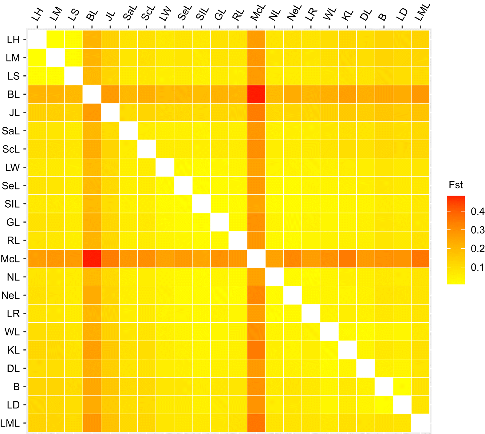
Three population differentiation analyses were used to examine subdivision among populations across the entire sampled range. First, we used GENODIVE to determine pairwise FST values between populations in all lakes (Supplementary Material 2, Table S3). Overall, comparisons among most lakes sampled from different sub-drainages resulted in significant FST values. Within each sub-drainage, the average FST values were 0.011 (SD = 0.003), 0.122 (SD = 0.077), 0.085 (SD = 0.104), and 0.060 (SD = 0.043) among populations in the Great Lakes, Winnipeg/Nelson, Churchill, and South Saskatchewan/Qu’appelle sub-drainages, respectively (Fig. 2; Supplementary Material 2, Table S3). Across sub-drainages, Winnipeg/Nelson and South Saskatchewan/Qu’appelle had the largest average FST values of 0.128 (SD = 0.066), followed by 0.114 (SD = 0.010) between Great Lakes and South Saskatchewan/Qu’appelle, 0.114 (SD = 0.097) between Winnipeg/Nelson and Churchill, 0.105 (SD = 0.052) between Great Lakes and Winnipeg/Nelson, 0.098 (SD = 0.062) between Great Lakes and Churchill, and 0.091 (SD = 0.077) between Churchill and South Saskatchewan/Qu’appelle (Fig. 2; Table S3). Fish in Mackay Lake in Saskatchewan showed the most differentiation from all other sites, with an average FST value of 0.299 (SD = 0.051), followed by Burt Lake with an average FST value of 0.232 (SD = 0.063). Some lakes in the Churchill River system (KL, NeL, and NL; see Table 1 for the list of site abbreviations) resulted in some comparisons that were not significant after Bonferroni correction (Supplementary Material 2, Table S3). Also, some comparisons including BL and LML had FST values that were not significant following Bonferroni correction, but this could be due to sample size as the comparisons still resulted in high FST values (Supplementary Material 2, Table S3).
Fig. 2.
Fig. 2. Heatmap representing the pairwise fixation indices (FST) from GENODIVE across all sample sites. Larger FST values represent larger population differentiation. This analysis was run after removing loci out of Hardy–Weinberg Equilibrium in 11 populations. Site abbreviations can be found in Table 1.
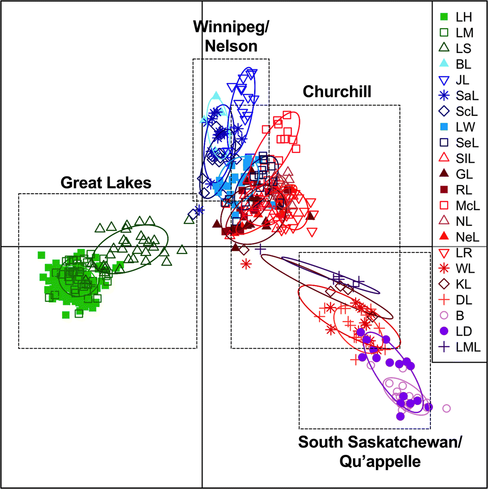
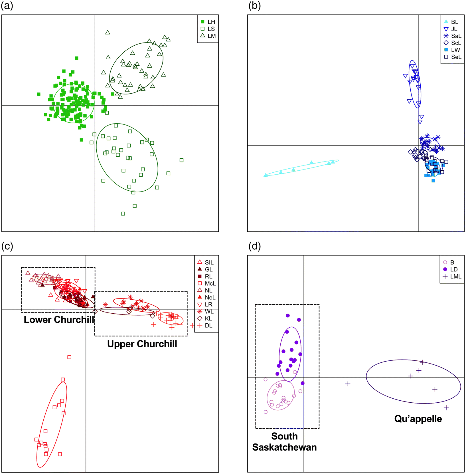
We ran DAPC with all sampled populations using 15 principal components as determined using the optim_a_score() function. Whitefish populations were significantly differentiated at different spatial scales both within and between provinces. This analysis broadly differentiated populations from the different lakes by sub-drainage and geographic distance along the first axis, explaining 39.2% of the variation. Specifically, along the first axis the Great Lakes were separated from the rest of the sites (Fig. 3). Lakes in the upper Churchill River (KL, DL and WL), South Saskatchewan River (B and LD), and Qu’appelle River (LML) were also differentiated along the first axis (Fig. 3). The second axis explained 15.3% of the variation and showed a gradient of variation by distance based on sub-drainage, with lakes in the Winnipeg and Nelson River sub-drainages differentiating from lakes in the Churchill River sub-drainage and South Saskatchewan and Qu’appelle sub-drainages (Fig. 3). The average assignment proportion of each individual in the broad analysis was high with a value of 0.892. Differentiation was also detected on sub-drainage scale, running the DAPC using 7 principal components in the Great Lakes, 6 in Lake Winnipeg/Nelson River, 8 in the Churchill River, and 3 in the South Saskatchewan and Qu’appelle sub-drainages (Fig. 4a–d). The first two axes in the Great Lakes analysis explain 52.3% and 47.7%, respectively, and separated each of the Great Lakes (Fig. 4a). The DAPC analysis of the Lake Winnipeg and Nelson River sub-drainages explained 29.7% along the first axis and separated BL and explained 27.5% along the second axis and differentiated JL (Fig. 4b). The first axis of the Churchill River sub-drainage explained 39.9% and differentiated upper and lower Churchill River samples, while the second axis explained 37.9% and separated McL (Fig. 4c). The Qu’appelle River and South Saskatchewan River samples were differentiated along the first axis of the DAPC analysis, explaining 85.2% and B and LD in the South Saskacthewan River sub-drainage were separated along the second axis, with 14.8% of the of the variation (Fig. 4d). When run independently, each sub-drainage had high assignment proportions with 0.980 in the Great Lakes, 1.000 in Lake Winnipeg/Nelson River, 0.864 in the Churchill River and 0.902 in South Saskatchewan/Qu’appelle.
Fig. 3.
Fig. 3. Discriminant analysis of principal components of all lakes in the study using 15 principal components as determined using the optim.a.score() function. Site abbreviations can be found in Table 1.
Fig. 4.
Fig. 4. Discriminant analysis of principal components analysis of (a) Great Lakes, (b) Lake Winnipeg and Nelson River sub-drainages, (c) Churchill River sub-drainage, and (d) South Saskatchewan River and Qu’appelle River sub-drainages. The optim.a.score() function was used to determine the optimal number of principal components was 7, 6, 8, and 3 for the analysis with the Great Lakes, Lake Winnipeg/Nelson River, Churchill and South Saskatchewan/Qu’appelle river basins, respectively. Site abbreviations can be found in Table 1.
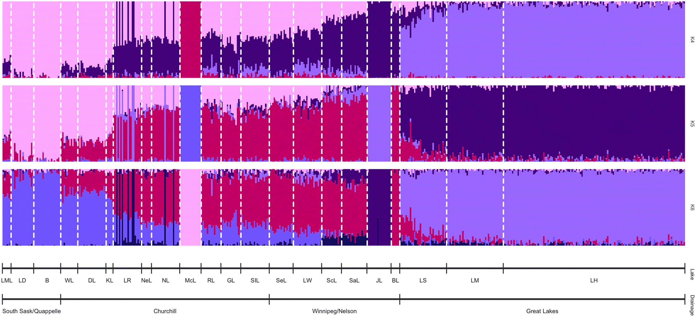
The optimal number of clusters (K) was determined using the cross-validation (CV) technique in ADMIXTURE. The three K values with the lowest CV were retained with K = 4 having a CV value of 0.512, K = 5 with a value of 0.511, and K = 6 with a value of 0.510. Importantly, all three K values detected a gradient of differentiation both on a broad and sub-drainage scale (Fig. 5). Each K value had high ancestry coefficients of 0.799 (SD = 0.200) for K = 4, 0.825 (SD = 0.147) for K = 5, and 0.808 (SD = 0.150) for K = 6 (Fig. 5). Further, within sub-drainages we detected differentiation based on hydrological connectivity and geographic distance between sampled populations. This differentiation reflected the results of the DAPC analysis with BL, JL, and McL showing differentiation from other lakes within their sub-drainage (Fig. 5). Within the Churchill sub-drainage there was a distinct gradient based on connectivity with populations from the upper Churchill River (KL, WL, and DL) slightly differentiating from those in the lower Churchill River (SIL, GL, RL, NL, NeL, and LR; Fig. 5). Similar to previous analyses, fish from McL strongly differentiated in all three K values with average ancestry coefficients of 0.999 (SD = 1.81 × 10⁻⁶), 0.999 (SD = 1.49 × 10⁻¹⁶), and 0.999 (SD = 0.00) for the K = 4, K = 5, and K = 6 data, respectively (Fig. 4). The Great Lakes populations sampled were differentiated from those at the other sites in Ontario with average ancestry coefficients of 0.922 (SD = 0.086) in K = 4, 0.905 (SD = 0.089) in K = 5, and 0.894 (SD = 0.090) in K = 6 (Fig. 5).
Fig. 5.
Fig. 5. ADMIXTURE analysis of all sampled lakes showing K = 4, K = 5, and K = 6 as determined using cross-validation. Each line represents an individual from the corresponding sample site. Site abbreviations can be found in Table 1.

Discussion

Lake whitefish showed broadscale population subdivision within the Mississippian lineage across central Canada and the United States. This is likely due to the lack of connectivity between distinct watersheds for thousands of years post-glaciation (Bernatchez and Dodson 1991). Differentiation based on geographic proximity alone was not supported by IBD analyses, indicating that the subdivision in populations across the sampled lakes is not just a simple function of IBD. Comparisons by sub-drainages were conducted to reflect hydrologic connectivity and in general resulted in larger FST values between river basins than within, even when covering large geographic regions. Large FST values within the Winnipeg/Nelson sub-drainage likely reflect the large geographic distance between lakes in this river basin, covering two large provinces, which reduces gene flow between populations and creates differentiation on a genomic level. Overall, we found evidence of structuring based on hydrological connectivity and watershed, which has not been previously investigated within the Mississippian lineage. Specifically, we found that hydrological connectivity based on sub-drainage enabled gene flow and reflected the differentiation observed among populations from the sampled sites (Table 1; Pringle 2003; Waples and Gaggiotti 2006).The level of differentiation found here was similar to previous studies examining population differentiation on similar spatial scales in other species including round whitefish (Morgan et al. 2017), Atlantic salmon (Moore et al. 2014), Atlantic cod (Bradbury et al. 2013), and the harbor porpoise (Lah et al. 2016). Morgan et al. (2017) examined round whitefish structure across North America and found similar levels of differentiation using pairwise FST comparisons on the same spatial scales as seen here. Although our fish all originated from the Mississippian refugium, we show distinct population differentiation across the sampled range, likely based on hydrological connectivity and corresponding levels of gene flow between sampled lakes.
Varying levels of differentiation were found within each of the sub-drainages, generally based on connectivity and distance. Overall, there was only a small gradient of differentiation within the Great Lakes, with evidence of higher genetic diversity downstream in Lake Huron, indicating that on a broad level the Great Lakes may be relatively connected. Lake Superior slightly differentiated from the rest of the Great Lakes. The importance of hydrology and associated connectivity among waterbodies for the evolution of genetic differences has been shown in previous population studies (Costello et al. 2003; Olsen et al. 2010; Morgan et al. 2017). The Great Lakes also showed a large amount of differentiation from the other sub-drainages, suggesting that despite profound anthropogenic influences, this system remains an important location for lake whitefish genetic diversity.
The largest amount of lake whitefish genetic diversity was found in the Churchill sub-drainage, where multiple clusters were observed in the DAPC analysis. Differentiation was found in the Churchill sub-drainage between lakes sampled in the upper Churchill River compared to those sampled further downstream. Due to the dendritic nature of rivers, lakes further downstream, such as LR and NL, result in higher genetic diversity from gene flow and migration (Crispo et al. 2006; Rougemont et al. 2020). This gradient of genetic diversity and differentiation was clear in the Churchill River, with lakes upstream, WL, KL and DL, clustering together, and those further downstream, NeL, NL, LR, RL, SIL, and GL, differentiating as well. Additionally, the lakes found further downstream had higher observed heterozygosity values than those found upstream, indicating that lakes further downstream have higher genetic diversity. The differentiation among populations may be a result of both geographic distance and environmental factors, with lakes found in different ecoregions, which may also be exposed to different environmental conditions (Rawson 1960). We also found that NeL, NL, and LR clustered together in all analyses; this is likely the result of connectivity because both NeL and NL drain into LR.
In contrast, Lake Diefenbaker and Blackstrap Lake are found in the South Saskatchewan River drainage, which passes through the highly agricultural regions of the Canadian prairies and collects 80% of the runoff from the Canadian Rockies (Gregor and Munawar 1989; Gober and Wheater 2014). Both of these lakes are manmade reservoirs that were filled in 1967 with the construction of the Gardiner Dam and supply drinking, irrigation, and industrial water supplies for some of the largest urban populations in the province (Hwang et al. 1975; Gober and Wheater 2014; Lucas et al. 2015). Whitefish from these lakes clustered together in the ordination and Bayesian analyses. This structuring could result from multiple factors including geographic proximity, both lakes are in the same sub-drainage and ecoregion, similar environmental conditions, or from founder effects resulting from stocking events (Gavrilets and Boake 1998; Laikre et al. 2010; Matute 2013). Further, fish found in these reservoirs are likely exposed to different environmental stressors as nutrient flow can be different as a result of irrigation and agriculture runoff (North et al. 2015; Sadeghian et al. 2015), and toxic substances have been found in the sediment (Gregor and Munawar 1989). Similar to the situation across provinces, it is likely that additional factors beyond simple distance and connectivity may influence population subdivision within Saskatchewan.
Although Mackay Lake is geographically close to Lac la Ronge, fish from this site were genetically distinct from those in Lac la Ronge in all three analyses, emphasizing the importance of hydrological connectivity. Upon inspection, MacKay Lake is located in a different sub-sub-drainage then other lakes sampled in the region, likely drastically reducing the connectivity between neighbouring lakes. Further, previous geological work from Maxeiner (1994) found that the composition of rocks near Mackay Lake varies from those in the Lac la Ronge area, likely resulting from the transition into the Boreal Shield ecozone. This geological change can drastically influence the productivity and composition of the lakes. Lake whitefish from Mackay Lake were also observed to have very low levels of heterozygosity, which may suggest a genetic bottleneck at some point since post-glacial colonization (Nei et al. 1975; Peery et al. 2012). Mackay Lake may only be very infrequently hydrologically connected to other waterbodies in the sub-sub-drainage, supporting the notion that it is potentially isolated, leading to the population differentiation and low heterozygosity observed in the dataset.

Limitations and future directions

In this study, we showed evidence for broad population structuring and differentiation across the Mississippian refugium. Due to our opportunistic sampling in Manitoba and Ontario, we were unable to sample as broadly as in Saskatchewan. Future studies should aim to examine genetic structuring within these provinces in more detail. The incorporation of genomic data allows for a better understanding of population structuring and can improve conservation and management of important species (von der Heyden 2017; Flanagan et al. 2018; Grummer et al. 2019; Xuerub et al. 2020). Future analyses should also aim to incorporate genomic markers that are under selection to further investigate population structuring and potentially examine local adaptation. The incorporation of non-neutral markers provides information on diversity and resilience and allows for better management and identification of populations that may require priority for conservation (von der Heyden 2017; Funk et al. 2019; Xuerub et al. 2020). It is important that future studies aim to strategically incorporate environmental variables that are likely influencing adaptation to fully understand population dynamics, such as gene flow and population structure (Flanagan et al. 2018; Grummer et al. 2019; Xuerub et al. 2020). Overall, future studies should include both neutral and non-neutral markers to best understand population differentiation and determine conservation units for management.

Conclusions

This study provides a novel perspective on the population structure of lake whitefish on multiple spatial scales in central Canada and the United States. The data support that geographic proximity and hydrological connectivity have the strongest influence on genetic population differentiation in the post-glacial environment. We found hierarchical structure at multiple geographic scales, first across sub-drainages where geographic distance restricts gene flow. Population subdivision on this scale was expected based on the period of isolation following glaciation, but the weak correlation in the IBD analysis indicates that forces beyond simple temporal and spatial isolation are also important. This finding may be informative for management as the identification of subdivision based on ecoregion and sub-drainage may aid in understanding appropriate scales for fisheries management. Currently, management of lake whitefish in Canada is undertaken by each province. Based on our findings, this level of management is appropriate to preserve larger patterns in genetic diversity and population differentiation. However, systems that span multiple political jurisdictions, especially near provincial boundaries, may require additional consideration for conservation of diversity on a larger scale. Overall, we found that barriers to gene flow based on hydrological connectivity (genetic drift) is one of the main factors driving population differentiation in lake whitefish. This study builds on previous work by Mee et al. (2015), by examining fine-scale differentiation in central Canada and the United States in the Mississippian lineage. With the current environmental pressures that could result in changes in hydrologic and environmental conditions, it is important to understand the adaptability, diversity, and subdivision across the entire range of the lake whitefish.

Funding statement

This work was supported by Natural Sciences and Engineering Research Council of Canada and Bruce Power Collaborative Research and Development Grants, awarded to JYW, CMS and RGM; the Canada Foundation for Innovation, McMaster University, the Northern Ontario School of Medicine, and the University of Regina.

Acknowledgements

We are very grateful to those agencies and personnel that contributed lake whitefish tissue samples for this work, including: the United States Geological Survey (Ann Arbor, MI), Saskatchewan Ministry of Environment’s Fisheries Unit, Manitoba Wildlife and Fisheries Branch, Ontario Ministry of Natural Resources and Forestry, and W. Larsen, University of Wisconsin, Stevens Point.

Competing interest statement

The authors declare no competing interests.

References

Alexander DH, Novembre J, and Lange K. 2009. Fast model-based estimation of ancestry in unrelated individuals. Genome Research, 19(9): 1655–1664.
Allendorf FW, Hohenlohe PA, and Luikart G. 2010. Genomics and the future of conservation genetics. Nature Reviews Genetics, 11: 697–709.
Andrews S. 2010. FastQC: A quality control tool for high throughput sequencing data [online]. Available from bioinformatics.babraham.ac.uk/projects/fastqc/.
Bence JR, Brenden TO, and Lijestrand EM. 2019. Feasibility of rehabilitating and supplementing fisheries by stocking lake whitefish in the Upper Great Lakes. White Paper Prepared for the Great Lakes Fishery Trust. Quantitative Fisheries Center, Michigan State University.
Bernatchez L, and Dodson JJ. 1990. Allopatric origin of sympatric populations of lake whitefish (Coregonus clupeaformis) revealed by mitochondrial-DNA restriction analysis. Evolution, 44(5): 1263–1271.
Bernatchez L, and Dodson J. 1991. Phylogeographic structure in mitochondrial DNA of the lake whitefish (Coregonus clupeaformis) and its relation to Pleistocene glaciations. Evolution, 45(4): 1016–1035.
Blanchet FG, Legendre P, and Bocard D. 2008. Forward selection of explanatory variables. Ecology, 89: 2623–2632.
Bolger AM, Lohse M, and Usadel B. 2014. Trimmomatic: A flexible read trimming tool for Illumina NGS data. Bioinformatics, btu170.
Bradbury IR, Hubert S, Higgins B, Bowman S, Borza T, Paterson IG, et al. 2013. Genomic islands of divergence and their consequences for the resolution of spatial structure in an exploited marine fish. Evolutionary Applications, 6: 450–461.
Brenden TO, Ebener MP, Sutton TM, Jones ML, Arts MT, Johnson TB, et al. 2010. Assessing the health of lake whitefish populations in the Laurentian Great Lakes: Lessons learned and research recommendations. Journal of Great Lakes Research, 36: 135–136.
Casselman JM, Collins JJ, Crossman EJ, Ihssen PE, and Spangler GR. 1981. Lake whitefish (Coregonus clupeaformis) stocks of the Ontario waters of Lake Huron. Canadian Journal of Fisheries and Aquatic Sciences, 38(12): 1772–1779.
Catchen J, Hohenlohe PA, Bassham S, Amores A, and Cresko WA. 2013. Stacks: An analysis tool set for population genomics. Molecular Ecology, 22: 3124–3140.
Costello AB, Down TE, Pollard SM, Pacas CJ, and Taylor EB. 2003. The influence of history and contemporary stream hydrology on the evolution of genetic diversity within species: An examination of microsatellite DNA variation in bull trout, Salvelinus confluentus (Pisces: Salmonidae). Evolution, 57(2): 328–344.
Crispo E, Bentzen P, Reznick DN, Kinnison MT, and Hendry AP. 2006. The relative influence of natural selection and geography on gene flow in guppies. Molecular Ecology, 15: 49–62.
Davey JW, Hohenlohe PA, Etter PD, Boone JQ, Catchen JM, and Blaxter ML. 2011. Genome-wide genetic marker discovery and genotyping using next-generation sequencing. Nature Reviews Genetics, 12: 499–510.
Department of Fisheries and Oceans Canada. 2016. Freshwater landings.
Dray S, Bauman D, Blanchet G, Borcard D, Clappe S, Guenard G, et al. 2021. adespatial: Multivariate multiscale spatial analysis. R package version 0.3-14. [online]: Available from CRAN.R-project.org/package=adespatial.
Dray S, Legendre P, and Peres-Neto PR. 2006. Spatial modelling: A comprehensive framework for principal coordinate analysis of neighbour matrices (PCNM). Ecological Modelling, 196(3-4): 483–493.
Dray S, and Dufour AB. 2007. The ade4 package: Implementing the duality diagram for ecologists. Journal of Statistical Software, 22(4): 1–20.
Eberner MP, Brenden TO, Wright GM, Jones ML, and Faisal M. 2010. Spatial and temporal distributions of lake whitefish spawning stocks in Northern lakes Michigan and Huron, 2003-2008. Journal of Great Lakes Research, 36: 38–51.
Eberner MP, Kinnunen RE, Schneeberger PJ, Mohr LC, Hoyle JA, and Peeters P. 2008. Managament of commercial fisheries for lake whitefish in the Laurentian Great Lakes of North America. International Governance of Fisheries Ecosystems, 99–143.
Excoffier L, Smouse PE, and Quattro JM. 1992. Analysis of molecular variance inferred from metric distances among DNA haplotypes: Application to human mitochondrial DNA restriction data. Genetics, 131: 479–491.
Excoffier L, Hofer T, and Foll M. 2009. Detecting loci under selection in a hierarchically structured population. Heredity, 103: 285–298.
Flanagan SP, Forester BR, Latch EK, Aitken SN, and Hoban S. 2018. Guidelines for planning genomic assessment and monitoring of locally adaptive variation to inform species conservation. Evolutionary Applications, 11: 1035–1052.
Foote CJ, Clayton JW, Lindsey CC, and Bodaly RA. 1992. Evolution of lake whitefish (Coregonus clupeaformis) in North America during the Pleistocene: Evidence for a Nahanni glacial refuge in the northern Cordilla region. Canadian Journal of Fisheries and Aquatic Sciences, 49: 760–768.
Forester BR, Lasky JR, Wagner HH, and Urban DL. 2018. Comparing methods for detecting multilocus adaptation with multivariate genotype-environment associations. Molecular Ecology, 27: 2215–2233.
Francis RM. 2016. POPHELPER: An R package and web app to analyse and visualize population structure. Molecular Ecology, 17(1): 27–32.
Franzin W, and Clayton J. 1977. A biochemical genetic study of zoogeaography of lake whitefish (Coregonus clupeaformis) in Western Canada. Journal of the Fisheries Research Board of Canada, 34(5): 617–625.
Funk WC, Forester BR, Converse SJ, Darst C, and Morey S. 2019. Improving conservation policy with genomics: A guide to integrating adaptive potential into U.S. Endangered Species Act decisions for conservation practitioners and geneticists. Conservation Genetics, 20: 115–134.
Gavrilets S, and Boake C. 1998. On the evolution of premating isolation after a founder event. The American Naturalist, 152(5): 706–716.
Gober P, and Wheater HS. 2014. Socio-hyrdrology and the science-policy interface: A case study of the Saskatchewan River basin. Hydrology and Earth System Sciences, 18: 1413–1422.
Gosselin T. 2018. grur: An R package tailored for RADseq data imputations.
Graham CF, Boreham DR, Manzon RG, Stott W, Wilson JY, and Somers CM. 2020. How “simple” methodological decisions affect interpretation of population structure based on reduced representation library DNA sequencing: A case study using the lake whitefish. PLOS ONE, e0226608.
Gregor DJ, and Munawar M. 1989. Assessing toxicity of Lake Diefenbaker (Saskatchewan, Canada) sediments using aalgal and nematode bioassays. Hydrobiologia, 188/189: 291–300.
Grummer JA, Beheregaray LB, Bernatchez L, Hand BK, Luikart G, Narum SR, and Taylor EB. 2019. Aquatic landscape genomics and environmental effects on genetic variation. Trends in Ecology and Evolution, 34(7): 641–654.
Hemmer-Hansen J, Therkildsen NO, and Pujolar JM. 2014. Population genomics of marine fishes: Next-generation prospects and challenges. Biological Bulletin, 227: 117–132.
Hwang CP, Huang PM, and Lackie TH. 1975. Phosphorus distribution in Blackstrap Lake sediments. Water Pollution Control Federation, 47(5): 1081–1086.
Isermann DA, Belnap MJ, Turnquist KN, Sloss BL, VanDeHey JA, Hansen SP, and Caroffino DC. 2020. Defining the need for genetic stock assignment when describing stock demographics and dynamics: An example using lake whitefish in Lake Michigan. Transactions of the American Fisheries Society, 149(4): 398–413.
Jombart T. 2008. adegenet: A R package for the multivariate analysis of genetic markers. Bioinformatics, 24(11): 1403–1405.
Jombart T, and Ahmed I. 2011. adegenet 1.3-1: New tools for the analysis of genome-wide SNP data. Bioinformatics, 27(21): 3070–3071.
Kinnunen RE. 2003. Great Lakes commercial fisheries. Michigan Sea Grant Extension, Michigan, USA.
Lah L, Trense D, Benke H, Berggren P, Gunnlaugsson P, Lockyer C, et al. 2016. Spatially explicit analysis of genome-wide SNPs detects subtle population structure in a mobile marine mammal, the harbor porpoise. PLoS ONE, 11(10): e0162792.
Laikre L, Schwartz MK, Waples RS, Ryman N, and The GeM Working Group. 2010. Compromising genetic diversity in the wild: Unmonitored large-scale release of plants and animals. Trends in Ecology and Evolution, 25(9): 520–529.
Larson WA, Isermann DA, and Feiner ZS. 2020. Incomplete bioinformatic filtering and inadequate age and growth analysis lead to an incorrect inference of harvest induced changes. Evolutionary Applications, 00: 1–12.
Lindsey CS, and Woods CC. 1970. Biology of coregonid fishes. University of Manitoba Press, Manitoba.
Liu L, Li Y, Hu N, He Y, Pong R, Lin D, Lu L, and Law M. 2012. Comparison of Next-generation sequencing systems. Journal of Biomedicine and Biotechnology, 2012: 251364.
Lu G, and Luo M. 2020. Genomes of major fishes in world fisheries and aquaculture: Status, application and perspective. Aquaculture and Fisheries, 5: 163–173.
Lucas BT, Liber K, and Doig LE. 2015. Spatial and temporal trends in reservoir physiochemistry and phosphorus speciation within Lake Diefenbaker, a Great Plains reservoir, as inferred from depositional sediments. Journal of Great Lakes Research, 41: 67–80.
Matute DR. 2013. The role of founder effects on the evolution of reproductive isolation. Journal of Evolutionary Biology, 26(11): 2299–2311.
Maxeiner RO. 1994. Geology of the MacKay Lake and Anglo Rouyn mine areas, southern La Ronge Domain (Part of NTS 73P-7). Summary of Investigations, Saskatchewan Geological Survey.
Mee JA, Bernatchez L, Reist JD, Rogers SM, and Taylor EB. 2015. Identifying designatable units for intraspecific conservation prioritization: A hierarchical approach applied to the lake whitefish species complex (Coregonus spp.). Evolutionary Applications, 8(5): 423–441.
Meirmans PG. 2020. GENODIVE version 3.0: Easy-to-use software for the analysis of genetic data of diploids and polyploids, Molecular Ecology Resources, 20: 1126–1131.
Moore JS, Bourret V, Dionne M, Bradbury I, O’Reilly P, Kent M, et al. 2014. Conservation genomics of anadromous Atlantic salmon across its North American range: Outlier loci identify the same pattern of population structure as neutral loci. Molecular Ecology, 23: 5680–5697.
Morgan TD, Graham CF, McArthur AG, Raphenya AR, Boreham DR, Manzon RG, et al. 2017. Genetic population structure of the round whitefish (Prosopium cylindraceum) in North America: Multiple markers reveal glacial refugia and regional subdivision. Canadian Journal of Fisheries and Aquatic Sciences, 75(6).
Nalepa TF, Mohr LC, Henderson BA, Madenjian CP, and Schneeberger PJ. 2005. Lake whitefish and Diporeia spp. in the Great Lakes: An overview. Proceedings of a Workshop on Dynamics of Lake Whitefish (Coregonus clupeaformis) and the amphipod Diporeia spp. in the Great Lakes. 3–19.
Nei M. 1987. Molecular Evolutionary Genetics. Columbia University Press, New York, NY.
Nei M, Maruyama T, and Chakraborty R. 1975. The bottlenck effect and genetic variability in populations. Evolution, 29(1): 1–10.
Nielsen EE, Hemmer-Hansen J, Larsen PF, and Bekkevold D. 2009. Population genomics of marine fishes: Identifying adaptive variation in space and time. Molecular Ecology, 18: 3128–3150.
North RL, Davies JM, Doig JE, Hudson JJ, and Lundenschmidt KE. 2015. Lake Diefenbaker: The prairie jewel. Journal of Great Lakes Research, 41: 1–7.
O’Leary SJ, Puritz JB, Willis SC, Hollenbeck CM, and Portnoy DS. 2018. These aren’t the loci you’re looking for: Principles of effective SNP filtering for molecular ecologists. Molecular Ecology, 27: 3193–3206.
Olsen JB, Beacham TD, Wetklo M, Seeb LW, Smith CT, Flannery BG, and Wenburg JK. 2010. The influence of hydrology and waterway distance on population structure of Chinook salmon Oncorhynchus tshawytcha in a large river. Journal of Fish Biology, 76: 1128–1148.
Ovenden JR, Berry O, Welch DJ, Buckworth RC, and Dichmont CM. 2015. Ocean’s eleven: A critical evaluation of the role of population, evolutionary and molecular genetics in the management of wild fisheries. Fish and Fisheries, 16: 125–129.
Papa Y, Oosting T, Valenza-Troubat N, Wellenreuther M, and Ritchie PA. 2020. Genetic stock structure of New Zealand dish and the use of genomics in fisheries management: An overview and outlook. New Zealand Journal of Zoology, 48.
Paris JR, Stevens JR, and Catchen JM. 2017. Lost in parameter space: A road map for Stacks. Methods in Ecology and Evolution, 8(10): 1360–1373.
Peery MZ, Kirby R, Reid BN, Stoelting R, Doucet-Beer E, Robinson S, et al. 2012. Reliability of genetic bottleneck tests for detecting recent population declines. Molecular Ecology, 21(14): 3403–3418.
Pringle C. 2003. What is hydrologic connectivity and why is it ecologically important? Hydrological Processes, 17: 2685–2689.
Purcell S, Neale B, Todd-Brown K, Thomas L, Ferreira MAR, Bender D, et al. 2007. PLINK: A tool set for whole-genome association and population-based linkage analyses. The American Journal of Human Genetics, 81: 559–575.
R Core Team. 2020. R: A language and environment for statistical computing. R Foundation for Statistical Computing, Vienna, Austria.
Rawson DS. 1960. A limnological comparison of twelve large lakes in northern Saskatchewan. Limnology and Oceanography, 5(2): 195–211.
Reitzel AM, Herrera S, Layden MJ, Martindale MQ, and Shank TM. 2013. Going where traditional markers have not gone before: Utility of and promise for RAD sequencing in marine invertebrate phylogeography and population genomics. Molecular Ecology, 22: 2953–2970.
Rennie MD, Sprules WG, and Johnson TB. 2009. Factors affecting the growth and condition of lake whitefish (Coregonus clupeaformis). Canadian Journal of Fisheries and Aquatic Sciences, 66(12): 2096–2108.
Renik KM, Jennings MJ, Kampa JM, Lyons J, Parks TP, and Sass GG. 2020. Status and distribution of cisco (Coregonus artedi) and lake whitefish (Coregonus clupeaformis) in inland lakes of Wisconsin. Northern Naturalist, 27(3): 469–484.
Rochette NC, and Catchen JM. 2017. Deriving genotypes from RAD-seq short-read data using Stacks. Nature Protocols, 12(12): 2640–2659.
Rougemont Q, Dolo V, Oger A, Besnard AL, Huteau D, Coutellec MA, et al. 2020. Riverscape genetic in brook lamprey: Genetic diversity is less influenced by river fragmentation than by gene flow with the anadromous ecotype. Heredity, 126: 235–250.
Russello MA, Waterhouse MD, Etter PD, and Johnson EA. 2015. From promise to practice: Pairing non-invasive sampling with genomics in conservation. PeerJ, e1106.
Sadeghian A, de Boer D, Hudson JJ, Wheater H, and Lindenschmidt KE. 2015. Lake Diefenbaker temperature model. Journal of Great Lakes Research, 41: 8–21.
Scott WB, and Crossman EJ. 1973. Freshwater fishes of Canada. Bulletin Fisheries Research Board of Canada. No. 184.
Stott W, VanDeHey JA, and Sloss BL 2010. Genetic diversity of lake whitefish in lakes Michigan and Huron; sampling, standardization, and research priorities. Journal of Great Lakes Research, 36: 59–65.
Stott W, Ebener MP, Mohr L, Hartman T, Johnson J, and Roseman EF. 2011. Spatial and temportal genetic diversity of lake whitefish (Coregonus clupeaformis (Mitchill)) from Lake Huron and Lake Erie. Advances in Limnology, 64: 205–222.
Valenzuela-Quinonez F. 2016. How fisheries management can benefit from genomics? Briefings in Functional Genomics, 15(5): 352–357.
VanDeHey JA, Sloss, BL, Peeters, PJ, and Sutton, TM. 2009. Genetic structure of lake whitefish (Coregonus clupeaformis) in Lake Michigan. Canadian Journal of Fisheries and Aquatic Sciences, 66(3): 382–393.
von der Heyden S. 2017. Making evolutionary history count: biodiversity planning for coral reef fishes and the conservation of evolutionary processes. Coral Reefs, 36: 183–194.
Vu NTT, Zenger KR, Guppy JL, Sellars MJ, Silva CN, Kjeldsen SR, and Jerry DR. 2020. Fine-scale population structure and evidence of local adaptation in Australian giant black tiger shrimp (Penaeus monodon) using SNP analysis. BMC Genomics, 21: 669.
Waples RS, and Gaggiotti O. 2006. What is a population? An empirical evaluation of some genetic methods for identifying the number of gene pools and their degree of connectivity. Molecular Ecology, 15: 1419–1439.
Wenne R, Boudry P, Hemmer-Hansen J, Lubieniecki KP, Was A, and Kause A. 2007. What role for genomics in fisheries management and aquaculture? Aquatic Living Resources, 20: 241–255.
Xuerub A, Benestan L, Normandeau E, Daigle RM, Curtis JMR, Bernatchez L, and Fortin MJ. 2018. Asymmetric oceanographic processes mediate connectivity and population genetic structure, as revealed by RADseq, in a highly dispersive marine invertebrate (Parastichopus californicus). Molecular Ecology, 27: 2347–2364.
Xuerub A, D’Aloia CC, Andrello M, Bernatchez L, and Fortin MJ. 2020. Incorporating putatively neutral and adaptive genomic data into marine conservation planning. Conservation Biology, 35(3): 909–920.
Zhou H, Alexander D, and Lange K. 2011. A quasi-Newtown acceleration for high-dimensional optimization algorithms. Statistics and Computing, 21: 261–273.

Supplementary material

Supplementary Material 1
Supplementary Material 2

Information & Authors

Information

Published In

cover image FACETS
FACETS
Volume 7Number 1January 2022
Pages: 853 - 874
Editor: Kristi M. Miller

History

Received: 7 December 2021
Accepted: 7 April 2022
Version of record online: 9 June 2022

Data Availability Statement

All relevant data are available from Dryad at https://doi.org/10.5061/dryad.p2ngf1vrf.

Key Words

  1. lake whitefish
  2. Mississippian lineage
  3. nextRAD
  4. SNPs
  5. population structure

Sections

Subjects

Authors

Affiliations

Carly F. Graham
Department of Biology, University of Regina, Regina, SK, Canada
Douglas R. Boreham
Medical Sciences, Northern Ontario School of Medicine, Greater Sudbury, ON, Canada
Richard G. Manzon
Department of Biology, University of Regina, Regina, SK, Canada
Joanna Y. Wilson
Department of Biology, McMaster University, Hamilton, ON, Canada
Christopher M. Somers [email protected]
Department of Biology, University of Regina, Regina, SK, Canada

Author Contributions

CFG and CMS conceived and designed the study.
CFG performed the experiments/collected the data.
CFG and CMS analyzed and interpreted the data.
DRB, RGM, JYW, and CMS contributed resources.
All drafted or revised the manuscript.

Metrics & Citations

Metrics

Other Metrics

Citations

Cite As

Export Citations

If you have the appropriate software installed, you can download article citation data to the citation manager of your choice. Simply select your manager software from the list below and click Download.

There are no citations for this item

View Options

View options

PDF

View PDF

Get Access

Media

Media

Other

Tables

Share Options

Share

Share the article link

Share on social media